


Next: Computational Considerations
Up: A Simple Scheme
Previous: Accuracy
Contents
Index
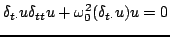
Beginning from the compact representation of the difference scheme given in (3.18), one may derive a discrete conserved energy similar to that obtained for the continuous problem in Section 3.1.2. Multiplying (3.18) by a discrete approximation to the velocity,
 gives
gives
 |
(3.34) |
Employing the product identities given in Section 2.4.2 in the last chapter, one may immediately arrive at
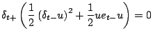 |
(3.35) |
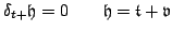
or
 |
(3.36) |
with
 |
(3.37) |
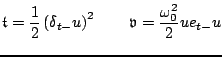
 and
and
 are clearly approximations to the kinetic and potential energies,
 and
and
 respectively, for the continuous problem, as defined in (3.10).
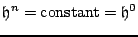
Equation (3.36) implies that the discrete time series
 , which approximates the total energy
 for the continuous time problem, is constant. Thus the scheme (3.18) is energy conserving, in a discrete sense. In other words,
 |
(3.38) |
Though one might think that the existence of a discrete conserved energy would immediately imply good behaviour of the associated finite difference scheme, just as in the continuous time case, it is important to note that the discrete approximation to potential energy, given above in (3.37), is not necessarily positive, and thus neither is
 . The determination of positivity conditions on
leads directly to a numerical stability condition. Expanding out the operator notation, one may write the function
at time step
. The determination of positivity conditions on
leads directly to a numerical stability condition. Expanding out the operator notation, one may write the function
at time step  as
as
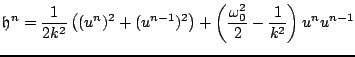 |
(3.39) |
which is no more than a quadratic form in the variables  and
and  . Applying the results given in §2.4.3, one may show that the quadratic form above is positive definite when
 |
(3.40) |
which is exactly the condition (3.25) arrived at through frequency domain analysis. Under this condition, one further has that
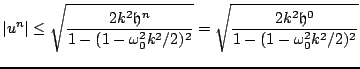 |
(3.41) |
Just as in the case of frequency domain analysis, the solution may be bounded in terms of the initial conditions (or the initial energy) and the system parameters. In fact, the bound above is identical to that given in (3.29). See Problem 3.11.
It is important to make some comments about the nature of this numerical energy conservation property. In infinite precision arithmetic, the quantity
remains exactly constant, according to (3.38). That is, the discrete kinetic energy
 and potential energy
 sum to the same constant, at any time step . See Figure 3.2(a). But in a finite precision computer implementation, there will be fluctuations in the total energy at the level of the least significant bit; such a fluctuation is shown, in the case of floating point arithmetic, in Figure 3.2(b). In this case, the fluctuations are on the order of
  of the total energy, and the bit-quantization of these variations is clearly visible. Thus energy is conserved to machine accuracy.
Figure:
(a) Variation of the discrete potential energy
 (solid grey line), discrete kinetic energy
 (dotted grey line) and total discrete energy
 (solid black line), plotted against time step , for the output of scheme (3.18). In this case, the values
 and
and  were used, and scheme (3.18) was initialized with the values
  and
and
 . (b) Variation of the error in energy, defined, at time step , as
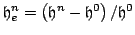 , plotted as black points. Multiples of single bit variation are plotted as grey lines.
|
The analysis of conservative properties of finite difference schemes is younger than frequency domain analysis, and, as a result, much less well-known. It is, however, far more powerful than the body of frequency domain analysis techniques which form the workhorse of scheme analysis. The energy method [102] is the name given to a class of analysis techniques which do not employ frequency domain concepts. The study of finite difference schemes which possess conservation properties (of energy, and other invariants) experienced a good deal of growth in the 1980s [101,188] and 1990s [139,244,91], and is related to more modern symplectic integration techniques [189,199].
Next: Computational Considerations
Up: A Simple Scheme
Previous: Accuracy
Contents
Index
Stefan Bilbao
2006-11-15