Frequency Domain Analysis

The frequency domain analysis of scheme (3.18) is very similar to that of the simple harmonic oscillator, as outlined in Section 3.1.1. Applying a $z$-transformation to (3.19), or, simply inserting a test solution of the form $u^n = z^n$, where $z = e^{sk}$, leads to the characteristic equation

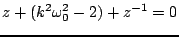$$z+(k^2 \omega_{0}^2-2)+z^{-1} = 0$$ (3.22)

which has the solution

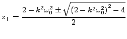$$z_{\pm} = \frac{2-k^2\omega_{0}^2\pm\sqrt{\left(2-k^2\omega_{0}^2\right)^2-4}}{2}$$ (3.23)

When $z_{\pm}$ are distinct, the solution to (3.18) will evolve according to

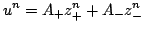$$u^n = A_{+}z_{+}^{n}+A_{-}z_{-}^n$$ (3.24)

Under the condition

$$k< \frac{2}{\omega_{0}}$$ (3.25)

the two roots $z_{\pm}$ will be complex conjugates of magnitude unity (see §2.3.3 and Problem 2.10), in which case they may be written as

$$z_{\pm} = e^{\pm j \omega k}$$ (3.26)

and the solution (3.24) may be rewritten as

$$u^n = A\cos(\omega n k)+B\sin(\omega n k) = C_{0}\cos(\omega n k + \phi_{0})$$ (3.27)

where

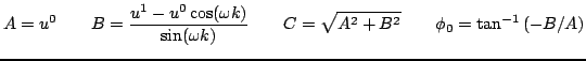$$A = u^{0}\qquad B = \frac{u^{1}-u^{0}\cos(\omega k)}{\sin(\omega k)}\qquad C = \sqrt{A^2+B^2}\qquad \phi_{0} = \tan^{-1}\left(-B/A\right)$$ (3.28)

This solution is clearly well-behaved, and resembles the solution to the continuous time SHO, from (3.3). From the form of (3.27), the following bound on the numerical solution size, in terms of the initial conditions and $\omega _{0}$ follows immediately:

$$\vert u^{n}\vert\leq C_{0}$$ (3.29)

Condition (3.25) may be violated in two different ways. If $k> \frac{2}{\omega_{0}}$, then the two roots of () will be real, and one will be of magnitude greater than unity. Thus solution (3.24) will clearly grow exponentially. If $k= \frac{2}{\omega_{0}}$, then the two roots of (3.23) coincide, at $z_{\pm} = -1$. In this case, the solution (3.24) does not hold, and there will be a term which grows linearly. In neither of the above cases does the solution behave in accordance with (3.3), and its size cannot be bounded in terms of initial conditions alone. Such growth is called numerically unstable (and in the latter case marginally unstable), and condition (3.25) serves as a stability condition.

Condition (3.25) may be rewritten, using sample rate $f_{s} = 1/k$ and oscillator frequency $f_{0} = \omega_{0}/2\pi$ as

$$f_{s}> \pi f_{0}$$ (3.30)

which, from the point of view of sampling theory, is counterintuitive. One would expect that the sampling rate necessary to simulate a sinusoid at frequency $f_{0}$ should satisfy $f_{s}>2 f_{0}$, not the above condition, which is more restrictive. The reason for this is of course that the numerical solution does not in fact oscillate at frequency $\omega _{0}$, but at frequency $\omega$ given by

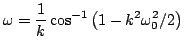$$\omega = \frac{1}{k}\cos^{-1}\left(1-k^2\omega_{0}^2/2\right)$$ (3.31)

This frequency warping effect is due to approximation error in the finite difference scheme (3.18) itself; such an effect will be generalized to numerical dispersion in distributed problems seen later in this book, and constitutes what is perhaps the largest single disadvantage of using time-domain methods for sound synthesis. Note in particular that $\omega > \omega_{0}$. Perceptually, such an effect will lead to mistuning of ``modes" in a simulation of a musical instrument. There are many means of combating this unwanted effect, perhaps the most crude being to use a higher sampling rate (or smaller value of $k$; note that frequency $\omega$ approaches $\omega _{0}$ in the limit as $k$ becomes small). This approach, however, though somewhat standard in the more mainstream simulation community, is not so useful in audio, as the sample rate is generally fixed^3.1. Another approach, which will be outlined in Section , involves different types of approximations to (3.1), and will be elaborated upon extensively throughout the rest of this book.