In §6.6, the ideal struck string was modeled as a simple initial velocity distribution along the string, corresponding to an instantaneous transfer of linear momentum from the striking hammer into the transverse motion of a string segment at time zero. (See Fig.6.10 for a diagram of the initial traveling velocity waves.) In that model, we neglected any effect of the striking hammer after time zero, as if it had bounced away at time 0 due to a so-called elastic collision. In this section, we consider the more realistic case of an inelastic collision, i.e., where the mass hits the string and remains in contact until something, such as a wave, or gravity, causes the mass and string to separate.
For simplicity, let the string length be infinity, and denote its wave
impedance by ![]() . Denote the colliding mass by
. Denote the colliding mass by ![]() and its speed
prior to collision by
and its speed
prior to collision by ![]() . It will turn out in this analysis that
we may approximate the size of the mass by zero (a so-called
point mass). Finally, we neglect the effects of gravity and
drag by the surrounding air. When the mass collides with the string,
our model must switch from two separate models (mass-in-flight and
ideal string), to that of two ideal strings joined by a mass
. It will turn out in this analysis that
we may approximate the size of the mass by zero (a so-called
point mass). Finally, we neglect the effects of gravity and
drag by the surrounding air. When the mass collides with the string,
our model must switch from two separate models (mass-in-flight and
ideal string), to that of two ideal strings joined by a mass ![]() at
at
![]() , as depicted in Fig.9.12. The ``force-velocity
port'' connections of the mass and two semi-infinite string endpoints
are formally in series because they all move together; that is,
the mass velocity equals the velocity of each of the two string
endpoints connected to the mass (see §7.2 for a fuller
discussion of impedances and their parallel/series connection).
, as depicted in Fig.9.12. The ``force-velocity
port'' connections of the mass and two semi-infinite string endpoints
are formally in series because they all move together; that is,
the mass velocity equals the velocity of each of the two string
endpoints connected to the mass (see §7.2 for a fuller
discussion of impedances and their parallel/series connection).
The equivalent circuit for the mass-string assembly after time zero is
shown in Fig.9.13. Note that the string wave impedance ![]() appears twice, once for each string segment on the left and right.
Also note that there is a single common velocity
appears twice, once for each string segment on the left and right.
Also note that there is a single common velocity ![]() for the two
string endpoints and mass. LTI circuit elements in series can be
arranged in any order.
for the two
string endpoints and mass. LTI circuit elements in series can be
arranged in any order.
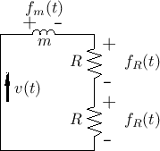 |
From the equivalent circuit, it is easy to solve for the velocity ![]() .
Formally, this is accomplished by applying Kirchoff's Loop Rule, which
states that the sum of voltages (``forces'') around any series loop is zero:
.
Formally, this is accomplished by applying Kirchoff's Loop Rule, which
states that the sum of voltages (``forces'') around any series loop is zero:
Taking the Laplace transform10.9of Eq.(9.8) yields, by linearity,
where
For the mass, we have
![$\displaystyle f_m(t) = m\,a(t)\;=\; m\,\frac{d}{dt} v(t) \quad\longleftrightarrow\quad
F_m(s) = m\left[s\,V(s) - v_0\right],
$](img2059.png)
where we used the differentiation theorem for Laplace transforms [452, Appendix D].10.10Note that the mass is characterized by its impedance
Substituting these relations into Eq.(9.9) yields
That is, an equivalent problem formulation is to start with the mass at rest and in contact with the string, followed by striking the mass with an ideal hammer (impulse) that imparts momentum
 |
An advantage of the external-impulse formulation is that the system
has a zero initial state, so that an impedance description
(§7.1) is complete. In other words, the system can be
fully described as a series combination of the three impedances ![]() ,
,
![]() (on the left), and
(on the left), and ![]() (on the right), driven by an external
force-source
(on the right), driven by an external
force-source
![]() .
.
Solving Eq.(9.10) for ![]() yields
yields
Since the Laplace transform of
We see that at time zero the mass velocity is
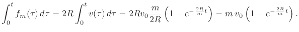
The displacement of the string at ![]() is given by the integral of
the velocity:
is given by the integral of
the velocity:
![$\displaystyle y(t,0) = \int_0^t v(\tau)\,d\tau = v_0\,\frac{m}{2R}\,\left[1-e^{-{\frac{2R}{m}t}}\right]
$](img2072.png)
where we defined the initial transverse displacement as
Thus, the final string displacement is proportional to both the ``hammer mass'' and the initial striking velocity; it is inversely proportional to the string wave impedance
The momentum of the mass before time zero is ![]() , and after time
zero it is
, and after time
zero it is
The force applied to the two string endpoints by the mass is given by
![]() . From Newton's Law,
. From Newton's Law,
![]() , we have that
momentum
, we have that
momentum ![]() , delivered by the mass to the string,
can be calculated as the time integral of applied force:
, delivered by the mass to the string,
can be calculated as the time integral of applied force:
Thus, the momentum delivered to the string by the mass starts out at zero, and grows as a relaxing exponential to
In a real piano, the hammer, which strikes in an upward (grand) or sideways (upright) direction, falls away from the string a short time after collision, but it may remain in contact with the string for a substantial fraction of a period (see §9.4 on piano modeling).
![\includegraphics[width=\twidth]{eps/massstringphy}](img2049.png)