Next |
Prev |
Up |
Top
|
JOS Index |
JOS Pubs |
JOS Home |
Search
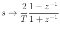
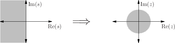
Wave Digital Filters are based on the application of a spectral mapping or bilinear transform:
which takes the  RHP to the
  outer disk:
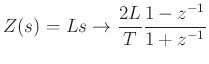
 is the time step and
 is the sampling frequency.
- Stable causal analog filters mapped to stable causal digital filters. Also: DC
 DC,
DC,
 Nyquist.
- Discrete ``impedances'' inherit passivity property (now called pseudo-passivity), and are called positive real in the outer disk.
Trapezoid Rule
In the time domain, this bilinear transform is equivalent to applying the trapezoid rule in order to integrate (or differentiate).
Connecting Digital N-ports
- Can connect digital one-ports using Kirchoff's Laws, and still have power conservation. If elements are pseudopassive, then so is a network constructed from such elements.
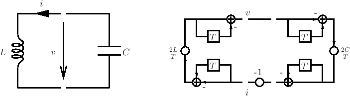
- Example: parallel
 connection
- Problem: Delay-free loops.
- Result: Signal-flow diagrams are non-realizable (unless one is willing to perform matrix inversions).
Wave Variables
It is possible to get around these realizability problems by
introducing wave variables (1971) borrowed from microwave
engineering
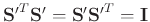
Introduce, for any port variables  and
and  , the quantities
 is an arbitrary positive constant, called the port resistance.
We can also define power-normalized wave variables as
is an arbitrary positive constant, called the port resistance.
We can also define power-normalized wave variables as
The two types of waves are simply related to eachother by
Power waves are useful in dealing with time-varying and nonlinear circuit elements.
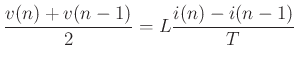
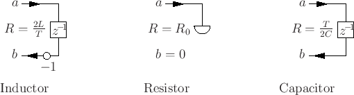
Example: Wave Digital Inductor
From the trapezoid rule (bilinear transform) we have
Inserting wave variables, we get:
And under the choice
 , we get
A strictly causal input/output relationship. (Same in power-normalized case).
- Energetic interpretation:
- Square of value in delay register has interpretation as stored energy
Wave-Digital Elements
We can derive wave digital equivalents of the standard circuit elements.
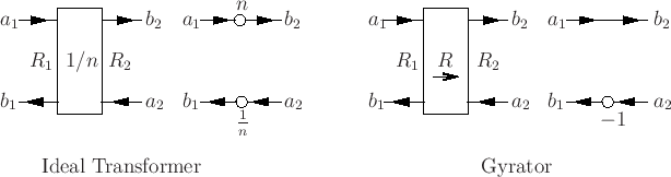
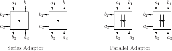
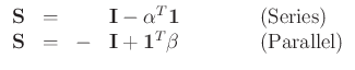
Adaptors
Connections between the elements are governed, as before, by Kirchoff's Laws. In terms of wave variables, we have, for a connection of  ports:
where
 is the conductance at port
  .
The signal processing block which carries out this operation is called an adaptor
.
The signal processing block which carries out this operation is called an adaptor
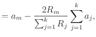
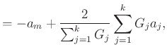
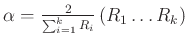
Scattering Matrices
The series and parallel adaptor equations can be written as
where
where
 ,
,
 we have also:
 in either case.
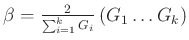
For power-normalized waves:
in either case.
For power-normalized waves:
where
 and
and
 (over all components).
We have
(over all components).
We have
 (orthonormal, unitary).
- Form of the adaptor equation is simple (O(N) adds, multiplies)
- Easy to apply rounding rules so that junction behaves passively, even in finite arithmetic:
- signals:Extended precision within junction. Magnitude truncation on outputs
- reflection parameters (
 ) may also be truncated without affecting passivity (though accuracy will of course suffer).
Next |
Prev |
Up |
Top
|
JOS Index |
JOS Pubs |
JOS Home |
Search
Download Meshes.pdf
Download Meshes_2up.pdf
Download Meshes_4up.pdf