The Membrane Shell

The simplest type of cylindrical shell theory is the membrane shell formulation of Rayleigh [77]. In this very basic theory, the shell is assumed to behave somewhat like a membrane, in that the restoring stiffness is assumed negligible. The shell is assumed to lie parallel to the $x$ axis, and has radius $a$. We define $\theta = a\theta'$, where $\theta'$ is the angular coordinate. This theory models the displacement of the shell from its equilibrium position; in contrast to Mindlin's plate system, however, displacements in all three directions are modeled as a function of time, and we will write these three displacements as $w_{z}$ (transverse), $w_{x}$ (axial) and $w_{\theta}$ (tangential). In the membrane theory, the three displacements complemented by three in-surface stresses $n_{x}$ (axial), $n_{\theta}$ (tangential) and $n_{x\theta}$ (shear) form a closed system; bending moments and transverse shear stresses are not modeled. This system can be written as

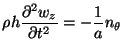$$\rho h\frac{\partial^{2}w_{z}}{\partial t^{2}} = -\frac{1}{a}n_{\theta}$$ (5.48)

$$\begin{eqnarray}\rho h\frac{\partial^{2}w_{x}}{\partial t^{2}} &=... ...heta}}{\partial x}+\frac{\partial w_{x}}{\partial \theta}\right) \end{eqnarray}$$ (5.49a)

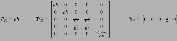
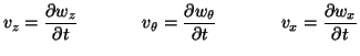
The material constants $E$, $\nu$, $\rho$ and the shell thickness $h$ are as discussed in §5.4, and are now assumed to be smooth functions of $x$ and $\theta$. If we define the velocities $v_{z}$, $v_{\theta}$ and $v_{x}$ by

$$v_{z} = \frac{\partial w_{z}}{\partial t}\hspace{0.5in}v_{\theta}... ... w_{\theta}}{\partial t}\hspace{0.5in}v_{x} = \frac{\partial w_{x}}{\partial t}$$

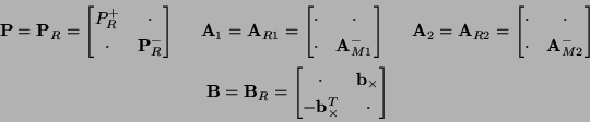
then we again have a symmetric hyperbolic system of the form of (3.1) in the dependent variable ${\bf w} = [v_{z}, v_{x}, v_{\theta}, n_{x}, n_{\theta}, n_{x\theta}]^{T}$, where the system matrices are

$$\begin{split}{\bf P} = {\bf P}_{R} = \begin{bmatrix}P_{R}^{+}... ...{\times}^{T} & \cdot\\ \end{bmatrix}\hspace{1.63in} \end{split}$$

where

$$P_{R}^{+} = \rho h\hspace{0.5in}{\bf P}_{R}^{-} = \begin{bmatrix}... ...ce{0.5in}{\bf b}_{\times} = \begin{bmatrix}0 &0&0&\frac{1}{a}&0\\ \end{bmatrix}$$

and ${\bf A}_{M1}^{-}$ and ${\bf A}_{M2}^{-}$ are as defined in (5.34) and (5.35). The lower 5 variable system described by ${\bf P}_{R}^{-}$, ${\bf A}_{R1}^{-}$ and ${\bf A}_{M2}^{-}$, when uncoupled from the 1 variable system in $P_{R}^{+}$ is essentially equivalent to the lower subsystem in the Mindlin plate theory, except that our independent variables are now $x$ and $\theta$ instead of $x$ and $y$. (In fact, if we replace any occurrence of $h^{3}/12$ in ${\bf P}_{M}^{-}$ by $h$, we get exactly ${\bf P}_{R}^{-}$.) We thus expect the MDKC to be very similar to that of the right-hand network in Figure 5.16.

We again introduce current-like variables

$$(i_{1},i_{9},i_{10},i_{11},i_{12},i_{13}) = (r_{1}v_{z},v_{x},v_{\theta},r_{4}n_{x}, r_{4}n_{\theta}, r_{5}n_{x\theta})$$

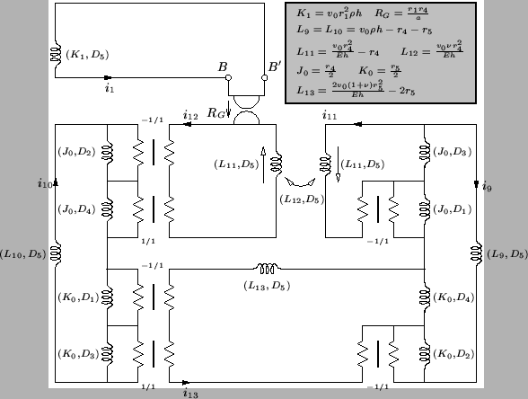
and make use of coordinates defined by (3.22) in terms of the physical coordinates $[x, \theta, t]^{T}$. $r_{1}$, $r_{4}$ and $r_{5}$ are, as before, positive constants which we will later use for optimization. The MDKC for the membrane shell system is shown in Figure 5.23. (We have marked the points $B$ and $B'$ in the figure in anticipation of the shell model in the next section.)

Figure 5.23: MDKC for the cylindrical membrane shell system.

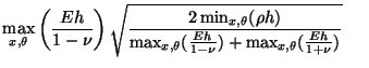
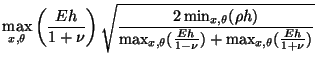
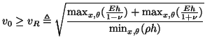
Optimal settings for $r_{4}$ and $r_{5}$, which follow from positivity constraints on the inductances $L_{9},\hdots,L_{13}$, can be shown (through an analysis identical to that performed on the Mindlin plate system) to be

$$r_{4} = \max_{x,\theta}\left(\frac{Eh}{1-\nu}\right)\sqrt{\frac{2\min_{x,... ..._{x,\theta}(\frac{Eh}{1-\nu})+\max_{x,\theta}(\frac{Eh}{1+\nu})}}\hspace{0.2in}$$ (5.50)

$$r_{5} = \max_{x,\theta}\left(\frac{Eh}{1+\nu}\right)\sqrt{\frac{2\min_{x,... ...(\rho h)}{\max_{x,\theta}(\frac{Eh}{1-\nu})+\max_{x,\theta}(\frac{Eh}{1+\nu})}}$$ (5.51)

in which case we must have, for passivity

$$v_{0}\geq v_{R}\triangleq \sqrt{\frac{\max_{x,\theta}(\frac{Eh}{1-\nu})+\max_{x,\theta}(\frac{Eh}{1+\nu})}{\min_{x,\theta}(\rho h)}}$$ (5.52)

The parameter $r_{1}$ is as yet unconstrained (notice that the inductance $K_{1}$ is non-negative for any choice of $v_{0}\geq 0$).

We have presented the MDKC for the membrane shell because it is an important building block in the more modern theory, which we now present. It should be obvious, from this MDKC, we can immediately arrive at an MDWD network, and after applying network transformations, we can get a multidimensional DWN as well.