


Next: A Second-order Family of
Up: Other Schemes
Previous: Other Schemes
Contents
Index
Another way to approximate (3.1) involves the use of temporal averaging operators, as introduced in Section 2.2. For example,
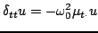 |
(3.42) |
is also a second order approximation to (3.1), where it is to be recalled that the averaging operator
 approximates the identity operation. Second order accuracy is easy enough to determine by inspection of the operator
 , which is a second order accurate approximation to
 .
.
This scheme, when the action of the operators
and
is expanded out, leads to
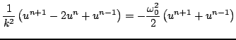 |
(3.43) |
which again involves values of the time series at three levels  ,
,  , and
, and  , and which can again be solved for
  , as
, as
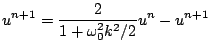 |
(3.44) |
The characteristic polynomial is now
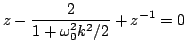 |
(3.45) |
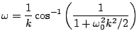
which has roots
 |
(3.46) |
The solution will again evolve according to (3.24) when  and
and  are distinct.
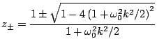
In this case, however, it is not difficult to show that the roots  will be complex conjugates of unit magnitude for any choice of
  . Thus
 , where the
  is given by
 |
(3.47) |
Again,
 , but, in contrast to the case of scheme (3.18), one now has
 . One now has a well-behaved sinusoidal solution of the form of (3.27) for any value of ; there is no stability condition of the form of (3.25).
The energetic analysis mirrors this behaviour. Multiplying (3.42) by
 gives
gives
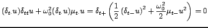 |
(3.48) |
or
 |
(3.49) |
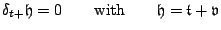
and
 |
(3.50) |
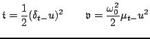
Now,
 and
and
 , and as a result
 are non-negative for any choice of . A bound on solution size follows immediately. See Problem 3.2.
Next: A Second-order Family of
Up: Other Schemes
Previous: Other Schemes
Contents
Index
Stefan Bilbao
2006-11-15