


Next: Hughes-Taylor and Newmark Methods
Up: Other Schemes
Previous: Using Time-averaging Operators
Contents
Index
A Second-order Family of Schemes
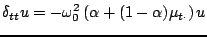
Though the stability condition inherent in scheme (3.18) has been circumvented in scheme (3.42), the problem of warped frequency persists. Using combination properties of the averaging operators, discussed in Section 2.2, it is not difficult to see that any scheme of the form
 |
(3.51) |
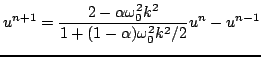
will also be a second-order accurate approximation to (3.1), for any choice of the real parameter  . In fact, it would be better to say ``at least second-order accurate"--see Section 3.3.4 for more discussion. There is thus a one-parameter family of schemes for (3.1), all of which operate as two step recursions: written out in full, the recursion has the form
 |
(3.52) |
Schemes (3.18) and (3.42) are members of this family with
 and
and
 , respectively.
It is interesting to examine the frequency warping characteristics of various members of this family, as function of
 , the reference frequency for the simple harmonic oscillator. In Figure 3.3, the frequency
  of the scheme (3.51) is plotted as a function of reference frequency
, for different choices of . Notice that for small values of , lower than about
of the scheme (3.51) is plotted as a function of reference frequency
, for different choices of . Notice that for small values of , lower than about
 , the difference scheme frequency is artificially low, and for values closer to , artificially high. In fact, for high values of , there is a certain ``cutoff" frequency
, for which the difference scheme becomes unstable--this is readily visible in the figure. In the middle range of values of (between about
and
, the difference scheme frequency is artificially low, and for values closer to , artificially high. In fact, for high values of , there is a certain ``cutoff" frequency
, for which the difference scheme becomes unstable--this is readily visible in the figure. In the middle range of values of (between about
and
 ), the difference scheme yields a good approximation over nearly the entire range of frequencies
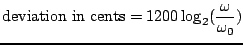
up to the Nyquist limit. It is useful, from a musical point of view, to plot the frequency deviation in terms of cents, defined as
), the difference scheme yields a good approximation over nearly the entire range of frequencies
up to the Nyquist limit. It is useful, from a musical point of view, to plot the frequency deviation in terms of cents, defined as
 |
(3.53) |
A deviation of 100 cents corresponds to a musical interval of a semitone.
which is shown in Figure 3.3(b). For low values of
Figure:
(a), frequency of the parameterized difference scheme (3.51) for the simple harmonic oscillator (3.1), plotted against
as dotted lines, for various values of the free parameter (indicated in the figure). The reference frequency is plotted as a solid black line. (b), deviation in cents of from
for the same members of the family, as a function of
![$ \omega _{0}\in [0, \frac {\pi }{k}]$](img45.png) . Zero deviation is plotted as a solid black line. Successive deviations of a musical semitone are indicated by grey horizontal lines.
. Zero deviation is plotted as a solid black line. Successive deviations of a musical semitone are indicated by grey horizontal lines.
 |
Next: Hughes-Taylor and Newmark Methods
Up: Other Schemes
Previous: Using Time-averaging Operators
Contents
Index
Stefan Bilbao
2006-11-15