An Exact Solution

For this very special case of the simple harmonic oscillator, there is in fact a two-step recursion which generates the exact solution to (3.1), at times $t=nk$. It is simply given by

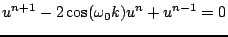$$u^{n+1}-2\cos(\omega_{0}k)u^{n}+u^{n-1}=0$$ (3.54)

This recursion is perhaps more familiar to electrical and audio engineers as a two-pole filter operating under transient conditions. The $z$ transformation analysis reveals:

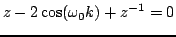$$z-2\cos(\omega_{0}k) + z^{-1} = 0$$ (3.55)

which has solutions

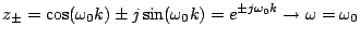$$z_{\pm} = \cos(\omega_{0}k)\pm j\sin(\omega_{0}k) = e^{\pm j\omega_{0}k} \rightarrow \omega = \omega_{0}$$ (3.56)

Thus the oscillation frequency $\omega$ of recursion (3.54) is exactly $\omega _{0}$, the frequency of the continuous time oscillator (3.1).

In a sense, then, all the preceding analysis of difference schemes is pointless, at least in the case of (3.1). On the other hand, the simple harmonic oscillator is a very special case; more complex systems, especially when nonlinear, rarely allow for exact numerical solutions. One other case of interest, however, and the main reason for dwelling on this point here, is the 1D wave equation, to be discussed in Chapter 6, which is of extreme practical importance in models of musical instruments which are essentially one-dimensional, such as strings and acoustic tubes. Numerical methods which are exact also exist in this case, and have been exploited with great success as digital waveguides [209].

Another question which arises here is that of accuracy. Considering again the one-parameter family of two-step difference schemes given by (3.51). Using identity (2.5) relating $\mu_{tt}$ to $\delta _{tt}$, it may be rewritten as

$$\delta_{tt}u = \frac{\omega_{0}^2}{1+\frac{\omega_{0}^2 (1-\alpha)k^2}{2}}u$$ (3.57)

Under the special choice of $\alpha = 1+\frac{2}{\omega_{0}^2}$, the difference scheme becomes exactly (3.54), or

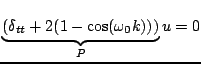$$\underbrace{\left(\delta_{tt}+2(1-\cos(\omega_{0}k))\right)}_{P}u=0$$ (3.58)

Consider the action of the operator $P$ as defined above on a continuous function. Expanding the operator $\delta _{tt}$ and the function $\cos(\omega_{0}k)$ in Taylor series leads to

$$P = \sum_{l=1}^{\infty}\frac{2 k^{2(l-1)}}{(2l)!}\frac{d^{2l}}{dt... ...k^{2(l-1)}}{(2l)!}\left(\frac{d^{2l}}{dt^{2l}}+(-1)^{l-1}\omega_{0}^{2l}\right)$$ (3.59)

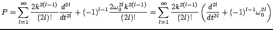
The various terms of the form $\left(\frac{d^{2l}}{dt^{2l}}+(-1)^{l-1}\omega_{0}^{2l}\right)$ all possess a factor of $\frac{d^{2}}{dt^{2}}+\omega_{0}^{2}$. Thus (3.58) may be rewritten as

$$\left(1+O(k^2)\right)\left(\frac{d^2}{dt^2}+\omega_{0}^2\right)u = 0$$ (3.60)

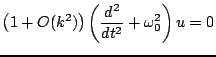
which shows that the solution $u$ indeed solves the equation of the simple harmonic oscillator exactly.

This property of accuracy of a difference scheme beyond that of the constituent operators, under very special choices of the scheme parameters, is indeed a very delicate one. In the distributed setting, it has been exploited in the construction of so-called modified equation methods [111,198,153,154,62] and compact spectral-like schemes [137,249,126,141].