Next |
Prev |
Up |
Top
|
Index |
JOS Index |
JOS Pubs |
JOS Home |
Search
Another versatile, effective, and often-used case is the
weighted least squares method, which is implemented in the
matlab function firls and others. A good general reference
in this area is [204].
Let the FIR filter length be  samples, with
  even, and suppose
we'll initially design it to be centered about the time origin (``zero
phase''). Then the frequency response is given on our frequency grid
even, and suppose
we'll initially design it to be centered about the time origin (``zero
phase''). Then the frequency response is given on our frequency grid
 by
by
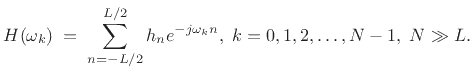 |
(5.33) |
Enforcing even symmetry in the impulse response, i.e.,
 , gives a zero-phase FIR filter that we can later right-shift
 samples to make a causal, linear phase filter. In this
case, the frequency response reduces to a sum of cosines:
samples to make a causal, linear phase filter. In this
case, the frequency response reduces to a sum of cosines:
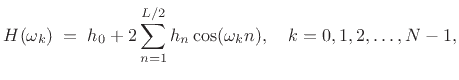 |
(5.34) |
or, in matrix form:
![$\displaystyle \underbrace{\left[ \begin{array}{c} H(\omega_0) \\ H(\omega_1) \\ \vdots \\ H(\omega_{N-1}) \end{array} \right]}_{{\underline{d}}} = \underbrace{\left[ \begin{array}{ccccc} 1 & 2\cos(\omega_0) & \dots & 2\cos[\omega_0(L/2)] \\ 1 & 2\cos(\omega_1) & \dots & 2\cos[\omega_1(L/2)] \\ \vdots & \vdots & & \vdots \\ 1 & 2\cos(\omega_{N-1}) & \dots & 2\cos[\omega_{N-1}(L/2)] \end{array} \right]}_\mathbf{A} \underbrace{\left[ \begin{array}{c} h_0 \\ h_1 \\ \vdots \\ h_{L/2} \end{array} \right]}_{{\underline{h}}} \protect$](img845.png) |
(5.35) |
Recall from §3.13.8, that the Remez multiple exchange
algorithm is based on this formulation internally. In that case, the
left-hand-side includes the alternating error, and the frequency grid
iteratively seeks the frequencies of maximum error--the
so-called extremal frequencies.
In matrix notation, our filter-design problem can be stated as (cf.
§3.13.8)
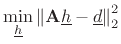 |
(5.36) |
where these quantities are defined in (4.35). We can denote the
optimal least-squares solution by
 |
(5.37) |
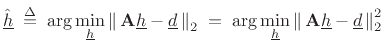
To find
 , we need to minimize
This is a quadratic form in
 . Therefore, it has a
global minimum which we can find by setting the gradient to
zero, and solving for
.5.14Assuming all quantities are real, equating the gradient to zero yields
the so-called normal equations
. Therefore, it has a
global minimum which we can find by setting the gradient to
zero, and solving for
.5.14Assuming all quantities are real, equating the gradient to zero yields
the so-called normal equations
 |
(5.39) |
with solution
![$\displaystyle \zbox {{\underline{\hat{h}}}\eqsp \left[(\mathbf{A}^T\mathbf{A})^{-1}\mathbf{A}^T\right]{\underline{d}}.}$](img855.png) |
(5.40) |
The matrix
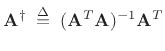 |
(5.41) |
is known as the (Moore-Penrose) pseudo-inverse of the matrix
 . It can be interpreted as an orthogonal projection
matrix, projecting
. It can be interpreted as an orthogonal projection
matrix, projecting
 onto the column-space of
[264], as we illustrate further in the next section.
onto the column-space of
[264], as we illustrate further in the next section.
Subsections
Next |
Prev |
Up |
Top
|
Index |
JOS Index |
JOS Pubs |
JOS Home |
Search
[How to cite this work] [Order a printed hardcopy] [Comment on this page via email]