When a white-noise sequence is filtered, successive samples generally become correlated.7.8 Some of these filtered-white-noise signals have names:
In the preceding sections, we have looked at two ways of analyzing noise: the sample autocorrelation function in the time or ``lag'' domain, and the sample power spectral density (PSD) in the frequency domain. We now look at these two representations for the case of filtered noise.
Let ![]() denote a length
denote a length ![]() sequence we wish to analyze. Then the
Bartlett-windowed acyclic sample autocorrelation of
sequence we wish to analyze. Then the
Bartlett-windowed acyclic sample autocorrelation of ![]() is
is ![]() ,
and the corresponding smoothed sample PSD is
,
and the corresponding smoothed sample PSD is
![]() (§6.7, §2.3.6).
(§6.7, §2.3.6).
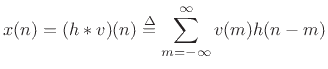
For filtered white noise, we can write ![]() as a convolution of white
noise
as a convolution of white
noise ![]() and some impulse response
and some impulse response ![]() :
:
 |
(7.29) |
| (7.30) |

since
![]() for white noise.
Thus, we have derived that the autocorrelation of filtered white noise
is proportional to the autocorrelation of the impulse response times
the variance of the driving white noise.
for white noise.
Thus, we have derived that the autocorrelation of filtered white noise
is proportional to the autocorrelation of the impulse response times
the variance of the driving white noise.
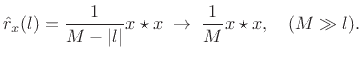
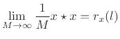
Let's try to pin this down more precisely and find the proportionality
constant. As the number ![]() of observed samples of
of observed samples of
![]() goes to infinity, the length-
goes to infinity, the length-![]() Bartlett-window bias
Bartlett-window bias ![]() in the autocorrelation
in the autocorrelation ![]() converges to a constant scale factor
converges to a constant scale factor
![]() at lags such that
at lags such that ![]() . Therefore, the unbiased
autocorrelation can be expressed as
. Therefore, the unbiased
autocorrelation can be expressed as
 |
(7.31) |
 |
(7.32) |
![\begin{eqnarray*}
S_x(\omega) &=&
\lim_{M\to \infty}\frac{1}{M}\vert X(\omega)\vert^2 \;=\;
% = \frac{1}{M}\vert H(\omega)\,V(\omega)\vert^2
\vert H(\omega)\vert^2 \cdot \lim_{M\to \infty} \frac{\vert V(\omega)\vert^2}{M} \\ [5pt]
&=&
\vert H(\omega)\vert^2 S_v(\omega) \;=\;
\vert H(\omega)\vert^2\sigma_v^2 \;\longleftrightarrow\;
(h\star h) \sigma_v^2 .
\end{eqnarray*}](img1190.png)
In summary, the autocorrelation of filtered white noise ![]() is
is
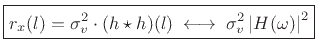 |
(7.33) |
In words, the true autocorrelation of filtered white noise equals the autocorrelation of the filter's impulse response times the white-noise variance. (The filter is of course assumed LTI and stable.) In the frequency domain, we have that the true power spectral density of filtered white noise is the squared-magnitude frequency response of the filter scaled by the white-noise variance.
For finite number of observed samples of a filtered white noise
process, we may say that the sample autocorrelation of filtered white
noise is given by the autocorrelation of the filter's impulse response
convolved with the sample autocorrelation of the driving white-noise
sequence. For lags ![]() much less than the number of observed samples
much less than the number of observed samples
![]() , the driver sample autocorrelation approaches an impulse scaled by
the white-noise variance. In the frequency domain, we have that the
sample PSD of filtered white noise is the squared-magnitude frequency
response of the filter
, the driver sample autocorrelation approaches an impulse scaled by
the white-noise variance. In the frequency domain, we have that the
sample PSD of filtered white noise is the squared-magnitude frequency
response of the filter
![]() scaled by a sample PSD of the
driving noise.
scaled by a sample PSD of the
driving noise.
We reiterate that every stationary random process may be defined, for our purposes, as filtered white noise.7.9 As we see from the above, all correlation information is embodied in the filter used.