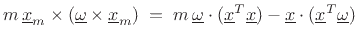
The two cross-products in Eq.(B.19) can be written out with the help of the vector analysis identityB.23
This (or a direct calculation) yields, starting with Eq.(B.19),
![$\displaystyle \mathbf{I}\underline{\omega}\eqsp
\left[\begin{array}{ccc}
I_{11} & I_{12} & I_{13}\\ [2pt]
I_{21} & I_{22} & I_{23}\\ [2pt]
I_{31} & I_{32} & I_{33}
\end{array}\right]
\left[\begin{array}{c} \omega_1 \\ [2pt] \omega_2 \\ [2pt] \omega_3\end{array}\right]
$](img2876.png)
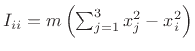
with
 , and
, and
The vector angular momentum of a rigid body is obtained by summing the angular momentum of its constituent mass particles. Thus,
Since
In summary, the angular momentum vector
![]() is given by the mass
moment of inertia tensor
is given by the mass
moment of inertia tensor
![]() times the angular-velocity vector
times the angular-velocity vector
![]() representing the axis of rotation.
representing the axis of rotation.
Note that the angular momentum vector
![]() does not in general
point in the same direction as the angular-velocity vector
does not in general
point in the same direction as the angular-velocity vector
![]() . We
saw above that it does in the special case of a point mass traveling
orthogonal to its position vector. In general,
. We
saw above that it does in the special case of a point mass traveling
orthogonal to its position vector. In general,
![]() and
and
![]() point
in the same direction whenever
point
in the same direction whenever
![]() is an eigenvector of
is an eigenvector of
![]() , as will be discussed further below (§B.4.16). In this
case, the rigid body is said to be dynamically balanced.B.24
, as will be discussed further below (§B.4.16). In this
case, the rigid body is said to be dynamically balanced.B.24
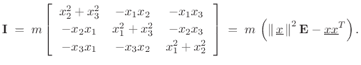
![$\displaystyle \mathbf{I}\eqsp m\left[\begin{array}{ccc}
x_2^2+x_3^2 & -x_1x_2 & -x_1x_3\\ [2pt]
-x_2x_1 & x_1^2+x_3^2 & -x_2x_3\\ [2pt]
-x_3x_1 & -x_3x_2 & x_1^2+x_2^2
\end{array}\right] \eqsp m\,\left(\left\Vert\,\underline{x}\,\right\Vert^2\mathbf{E}- \underline{x}\underline{x}^T\right).
\protect$](img2880.png)