| (44) |
Let us now approach the simulation of propagation in lossy media which are represented by equation (26). We treat the one-dimensional scalar case here in order to focus on the kinds of filters that should be designed to embed losses in digital waveguide networks [44,25].
As usual, by inserting the exponential eigensolution into the wave
equation, we get the one-variable version of (29)
Reconsidering the treatment of section III-A and reducing
it to the scalar case, let us derive from (33)
and (34) the expression for
![]()
If the frequency range of interest is above a certain threshold, i.e.,
![]() is small, we can obtain the following
relations from (47), by means of a Taylor expansion
truncated at the first term:
is small, we can obtain the following
relations from (47), by means of a Taylor expansion
truncated at the first term:
Still under the assumption of small losses, and truncating the Taylor
expansion of ![]() to the first term, we find that the wave
admittance (35) reduces to the two ``directional
admittances'':
to the first term, we find that the wave
admittance (35) reduces to the two ``directional
admittances'':
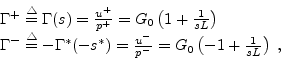
The actual wave admittance of a one-dimensional medium, such as a tube, is ![]() while
while
![]() is its paraconjugate in the analog domain. Moving to the discrete-time domain by means of a bilinear transformation, it is easy to verify that we get a couple of ``directional admittances'' that are related through (21).
is its paraconjugate in the analog domain. Moving to the discrete-time domain by means of a bilinear transformation, it is easy to verify that we get a couple of ``directional admittances'' that are related through (21).
In the case of the dissipative tube, as we expect, wave propagation is not lossless, since
![]() . However, the medium is passive in the sense of section II-E, since the sum
. However, the medium is passive in the sense of section II-E, since the sum
![]() is positive semidefinite along the imaginary axis.
is positive semidefinite along the imaginary axis.
The relations here reported hold for any one-dimensional resonator with frictional losses. Therefore, they hold for a certain class of dissipative strings and tubes. Remarkably similar wave admittances are also found for spherical waves propagating in conical tubes (see Appendix A).
The simulation of a length-![]() section of lossy resonator can proceed according to two stages of approximation. If the losses are small (i.e.,
section of lossy resonator can proceed according to two stages of approximation. If the losses are small (i.e.,
![]() ) the approximation (48) can be considered valid in all the frequency range of interest. In such case, we can lump all the losses of the section in a single coefficient
) the approximation (48) can be considered valid in all the frequency range of interest. In such case, we can lump all the losses of the section in a single coefficient
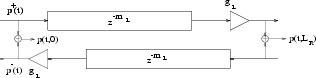
![]() . The resonator can be simulated by the structure of Fig. 3, where we have assumed that the length
. The resonator can be simulated by the structure of Fig. 3, where we have assumed that the length ![]() is equal to an integer number
is equal to an integer number ![]() of spatial samples.
of spatial samples.
At a further level of approximation, if the values of
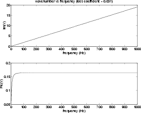
On the other hand, if losses are significant, we have to represent wave propagation in the two directions with a filter whose frequency response can be deduced from Fig. 2.
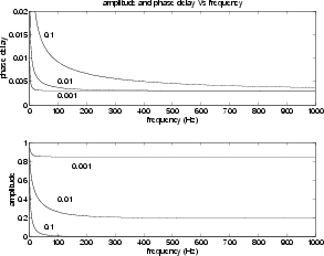
In practice, we have to insert a filter ![]() having magnitude and phase delay that are represented in Fig. 4 for different values of
having magnitude and phase delay that are represented in Fig. 4 for different values of ![]() . From such filter we can subtract a contribution of linear phase, which can be implemented by means of a pure delay.
. From such filter we can subtract a contribution of linear phase, which can be implemented by means of a pure delay.
 |