Distributed Problems and Coordinate Changes

Symmetric Hyperbolic Systems

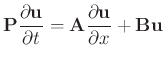
Multidimensional time and space-dependent physical systems are often described by systems of PDEs which are symmetric hyperbolic. For example, in 1D, a typical situation is:

$${\bf P}\frac{\partial {\bf u}}{\partial t} = {\bf A}\frac{\partial {\bf u}}{\partial x} + {\bf Bu}$$

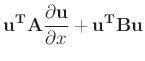
where ${\bf P(x)}$ is symmetric, $>0$ , and ${\bf A(x)}$ is symmetric (both square, real). Can write:

$${\bf u^{T}P}\frac{\partial {\bf u}}{\partial t} = {\bf u^{T}A}\frac{\partial {\bf u}}{\partial x} + {\bf u^{T}Bu}$$

$$\frac{1}{2}\frac{\partial {\bf u^{T}P u}}{\partial t} = \frac{1}{2}\frac{\partial {\bf u^{T}Au}}{\partial x} -\frac{1}{2}u^{T}\frac{\partial {\bf A}}{\partial x}u + \frac{1}{2}{\bf u^{T}(B+B^{T})u}$$

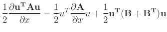
and integrating over the real line (assuming no boundaries,

$$\frac{\partial}{\partial t}\int_{x}{\bf u^{T}Pu}dx = \int_{x}{\bf u^{T}\left(-A'+B+B^{T}\right)u}$$

• $\int_{x}{\bf u^{T}Pu}dx$ is usually called the total energy of the system.
• like an ODE describing evolution of energy.
• if right-hand side is zero, then the system is lossless (in weighted ${\bf P}$ norm).
• if right-hand side is never positive, then the energy can only decrease.
• symmetric hyperbolic $\rightarrow$ reciprocal networks (almost).

CFL Criterion

Hyperbolic systems $\rightarrow$ finite propagation speeds.

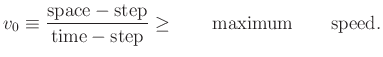
For explicit numerical methods on a grid, have a necessary stability condition on the time-step space-step ratio. In 1D, on a regular grid, only neighboring points:

$$v_{0}\equiv \frac{{\rm space-step}}{{\rm time-step}}\geq\qquad{\rm maximum\qquad speed.}$$

(Courant-Friedrichs-Lewy Condition).

In higher-D, same general result, but extra factors appear (solution does not necessarily move along a grid direction).

In the network approaches, CFL appears in an elementary way as a constraint on the positivity of the circuit elements (for passivity).

Multidimensional Problems and Coordinate Transformation

Multidimensional (distributed) systems $\rightarrow$ system of PDEs.

Time-dependent systems derived from conservation laws:

• may be of hyperbolic type (finite speeds)
• quantities conserved with respect to time alone.

In order to obtain a multidimensional circuit representation of a system of PDEs, useful to consider coordinate changes

$${\bf u}=({\bf x},t)^{T}\rightarrow {\bf t} = (t_{1}\hdots t_{k})^{T}$$

New coordinates should be causal, in the sense that:

• Any positive change $\Delta t$ in the variable $t$ (time) must be reflected by a similar positive change $\Delta t_{i}$ in all the new coordinates $t_{i}$ , $i=1\hdots k$ .
• Conversely, any positive change $\Delta t_{i}$ in any of the new coordinates must produce a positive change in the time variable $t$ .

A simple set of linear coordinate transformations:

$${\bf t} = {\bf H}^{-1}{\bf Vu}$$

• ${\bf V}$ is a diagonal square matrix of the form diag $(1,\hdots,v_{0})$ used to nondimensionalize the original coordinates. $v_{0}$ has dimension of a velocity.
• ${\bf H}$ is a square (preferably orthonormal) matrix. Elements in bottom row are all positive (to satisfy above criteria).

Remarks: A theoretical ``hack'' for extending passivity ideas to multi-D

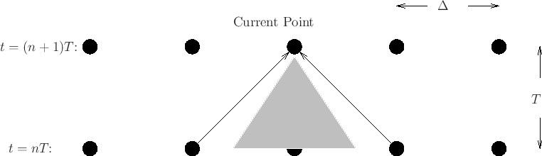
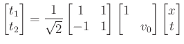
A Simple Coordinate Change and Sampling

If we have only one spatial dimension, then coordinate change options are limited. The only suitable one (in this context) is

$$\begin{bmatrix}t_{1}\\ t_{2}\\ \end{bmatrix}=\frac{1}{\sqrt{2}}\begin{bmatrix}1 &1\\ -1 & 1\\ \end{bmatrix} \begin{bmatrix}1 &\\ & v_{0}\\ \end{bmatrix} \begin{bmatrix}x\\ t\\ \end{bmatrix}$$

A simple rotation of the coordinates by 45 degrees. If we now define uniform grids in the two coordinate systems, we get:

• grid spacings $(\Delta, \frac{1}{v_{0}}\Delta)$ in original coordinates, $(T_{1}, T_{2}=T_{1})$ in new.
• grids partially align, if we have $T_{1} = \sqrt{2}\Delta$ .

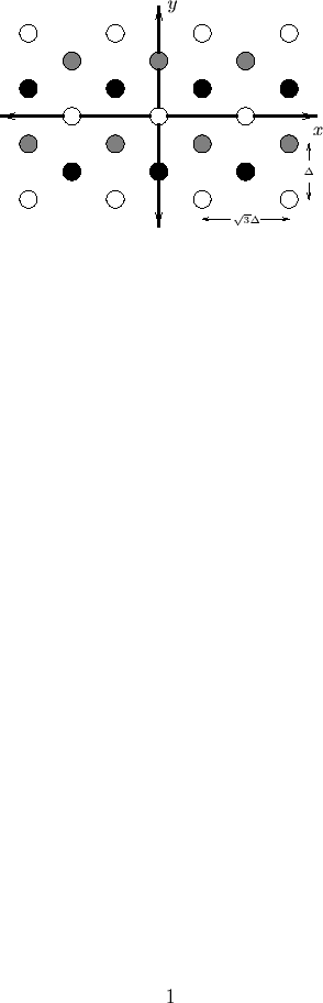
Coordinate Changes in Higher Dimensions: Hexagonal Coordinates

The transformation defined by

$$\mathbf{H} = \begin{bmatrix}\frac{1}{\sqrt{2}}&-\frac{1}{\sqrt{2}}&0\\ \frac{1}{\sqrt{6}}&\frac{1}{\sqrt{6}}&-\sqrt{\frac{2}{3}}\\ \frac{1}{\sqrt{3}}&\frac{1}{\sqrt{3}}&\frac{1}{\sqrt{3}}\\ \end{bmatrix}$$

when uniformly ``sampled'' in the new coordinates gives rise to the following grid pattern (viewed in the original coordinate system):

Three different grids (white, grey, black points) which exist every third time step.

Rectangular coordinates

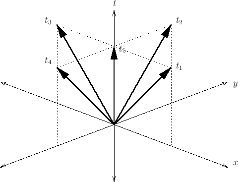
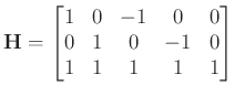
In order to generate a standard rectangular grid by uniformly sampling in the causal coordinates, need to use an embedding:

$$\mathbf{H} = \begin{bmatrix}1&0&-1&0&0\\ 0&1&0&-1&0\\ 1&1&1&1&1 \end{bmatrix}$$

which maps $(x,y,t)$ to a 5-dimensional space ${\bf t}$ = (north+time , south+time , east+time, west+time, time alone), and we get a normal rectangular grid in $(x,y)$ if we sample uniformly in the five directions

• Ugly theoretical manipulation to do something simple; not actually going to solve a problem in 5D. Need them to define directions of energy flow.
• Now need to define a particular right pseudo-inverse ${\bf H^{-R}}$ ...in practice, choice is relatively immaterial (but still must have elements of right column positive).
• Crux is: need five dimensions for a rectilinear grid, because in a simulation, energy can approach a grid point from any of the four compass points (and also from a past grid point at the same location).
• in 3D need to embed in a 7-D system.

Picture is: