Example: Bridge Coupling of Piano Strings

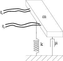
As an application of the theory, we outline the digital simulation of two pairs of piano strings. The strings are attached to a common bridge which acts as a coupling element between the strings (see Fig. 3). An in-depth treatment of coupled strings can be found in [132].

To a first approximation, the bridge can be modeled as a lumped mass-spring-damper system, while for the strings, a distributed waveguide representation is more appropriate. For the purpose of illustrating the theory in its general form, we represent each pair of strings as a single 2-variable waveguide. This approach is justified if we associate the pair with the same key in such a way that both the strings are subject to the same excitation. Since the $2 \times 2$ matrices $\mbox{\boldmath$M$}$ and ${\mbox{\boldmath$T$}}$ of (5) can be considered to be diagonal in this case, we could alternatively describe the system as four separate scalar waveguides.

Figure 3: Two pairs of strings coupled at a bridge.

The $i^{th}$ pair of strings is described by the $2$-variable impedance matrix

$${\mbox{\boldmath$R$}}_i = \left[ \begin{array}{cc} {R_{i,1}} & 0 \\ 0 & {R_{i,2}} \\ \end{array} \right]$$ (51)

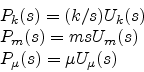
The lumped elements forming the bridge are connected in series, so that the driving-point velocity⁷ $u$ is the same for the spring, mass, and damper:

$$u(t)=u_m(t)=u_k(t)=u_{\mu}(t)$$ (52)

Also, the forces provided by the spring, mass, and damper, sum:

$$p(t)=p_m(t)+p_k(t)+p_{\mu}(t)$$ (53)

We can derive an expression for the bridge impedances using the following relations in the Laplace-transform domain:

$$\begin{array}{l} \displaystyle P_k(s)=(k/s) U_k(s)\\ P_m(s)={m s}U_m(s)\\ P_{\mu}(s)=\mu U_{\mu}(s)\\ \end{array}$$ (54)

Equations (55) and (54) give the continuous-time load impedance

$$R_L(s) = \frac{P(s)}{U(s)} = m\frac{s^2 + s \mu/m + k/m}{s}$$ (55)

In order to move to the discrete-time domain, we may apply the bilinear transform

$$s \leftarrow \alpha \frac{1 - z^{-1}}{1 + z^{-1}}$$ (56)

to (56). The factor $\alpha$ is used to control the compression of the frequency axis. It may be set to $2/T$ so that the discrete-time filter corresponds to integrating the analog differential equation using the trapezoidal method, or it may be chosen to preserve the resonance frequency (preferred).

We obtain

$$R_L(z) = \left[ (\alpha^2 - \alpha \mu/m + k/m)z^{-2} \right.$$

$$+ (-2 \alpha^2 + 2 k/m)z^{-1}$$

$$+ \left. (\alpha^2 + \alpha \mu/m + k/m) \right] \left/ \left[ \alpha / m (1 - z^{-2}) \right] \right.$$

The factor $S$ in the impedance formulation of the scattering matrix (48) is given by

$$S(z) = \left[ {\displaystyle \sum_{i,j=1}^{2}{R_{i,j}} } + R_L(z) \right]^{-1}$$ (57)

which is a rational function of the complex variable $z$. The scattering matrix is given by

$${\mbox{\boldmath$A$}}= 2 S \left[ \begin{array}{llll} {R_{1,... ...}} & {R_{2,2}} \\ \end{array} \right] - {\mbox{\boldmath$I$}}$$ (58)

which can be implemented using a single second-order filter having transfer function (58).