A straightforward multivariable generalization of the telegrapher's
equations (2) and (3) gives the following ![]() -variable
generalization of the wave equation (5):
-variable
generalization of the wave equation (5):
![\( {\mbox{\boldmath$x$}}^T \stackrel{\triangle}{=}
\left[
\begin{array}{lll}
x_1 & \dots & x_m
\end{array} \right]
\)](img40.png) at time
at time ![\begin{displaymath}
\left[ \frac{\partial^2{\mbox{\boldmath$p$}}({\mbox{\boldmat...
...{\mbox{\boldmath$x$}},t)}{\partial x_m^2}
\end{array}\right]
\end{displaymath}](img44.png) |
(6) |
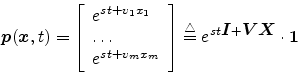
For digital waveguide modeling, we desire solutions of the multivariable
wave equation which involve only sums of traveling waves, because traveling
wave propagation can be efficiently simulated digitally using only delay
lines, digital filters, and scattering junctions. Consider the
eigenfunction
 ,
,
![${\mbox{\boldmath$V$}}{\tiny\stackrel{\triangle}{=}}\hbox{diag}([v_1, \ldots, v_m])$](img50.png) is a diagonal
matrix of spatial
Laplace-transform variables (the imaginary part of
is a diagonal
matrix of spatial
Laplace-transform variables (the imaginary part of ![${\mbox{\boldmath$1$}}^T {\tiny\stackrel{\triangle}{=}}[1,
\ldots, 1]$](img53.png) . Substituting the eigenfunction (7) into
(5) gives the algebraic equation
. Substituting the eigenfunction (7) into
(5) gives the algebraic equation
Having established that (10) is a solution of
(5) when condition (8) holds for the matrices
![]() and
and
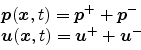
![]() , we can express the general traveling-wave
solution to (5) in both pressure and velocity as
, we can express the general traveling-wave
solution to (5) in both pressure and velocity as
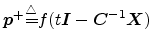 , with
 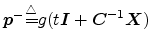 is similarly any linear combination of left-going eigensolutions from
(10) (all having the plus sign). Similar definitions apply for
is similarly any linear combination of left-going eigensolutions from
(10) (all having the plus sign). Similar definitions apply for
When the mass and stiffness matrices
![]() and
and
![]() are diagonal, our analysis corresponds to considering
are diagonal, our analysis corresponds to considering ![]() separate
waveguides as a whole. For example, the three directions of vibration
(one longitudinal and two transverse) in
a single terminated string can be described by
(5) with
separate
waveguides as a whole. For example, the three directions of vibration
(one longitudinal and two transverse) in
a single terminated string can be described by
(5) with ![]() . The coupling among the strings occurs
primarily at the bridge in a piano [132]. As we will see
later, the bridge acts like a junction of several multivariable
waveguides.
. The coupling among the strings occurs
primarily at the bridge in a piano [132]. As we will see
later, the bridge acts like a junction of several multivariable
waveguides.
When the matrices
![]() and
and
![]() are
non-diagonal, the physical interpretation can be of the form
are
non-diagonal, the physical interpretation can be of the form
Note that the multivariable wave equation (5) considered here
does not include wave equations governing propagation in multidimensional
media (such as membranes, spaces, and solids). In higher dimensions, the
solution in the ideal linear lossless case is a superposition of waves
traveling in all directions in the ![]() -dimensional
space [60]. However, it turns out [122]
that a good simulation of wave
propagation in a multidimensional medium may be in fact be obtained by
forming a mesh of unidirectional waveguides as considered here, each
described by (5). Such a mesh of 1D
waveguides can be shown to solve numerically a discretized wave equation
for multidimensional media [125].
-dimensional
space [60]. However, it turns out [122]
that a good simulation of wave
propagation in a multidimensional medium may be in fact be obtained by
forming a mesh of unidirectional waveguides as considered here, each
described by (5). Such a mesh of 1D
waveguides can be shown to solve numerically a discretized wave equation
for multidimensional media [125].