,
where `
,
where `
From the multivariable generalization of (2), we have, using
(10),
,
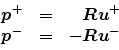
where `![]() ' is for right-going and `
' is for right-going and `![]() ' is for left-going. Thus,
following the classical definition for the scalar case, the wave impedance
is defined by
' is for left-going. Thus,
following the classical definition for the scalar case, the wave impedance
is defined by
More generally, when there is a loss represented by a diagonal matrix
![]() ,
we have, in the continuous-time case,
,
we have, in the continuous-time case,
 as before, leading to the admittance matrix
A linear propagation medium in the discrete-time case is completely
determined by its wave impedance
![]() (generalized here to
permit frequency-dependent and spatially varying wave impedances). A waveguide is defined for purposes of this paper as a length of medium in
which the wave impedance is either constant with respect to spatial
position
(generalized here to
permit frequency-dependent and spatially varying wave impedances). A waveguide is defined for purposes of this paper as a length of medium in
which the wave impedance is either constant with respect to spatial
position ![]() , or else it varies smoothly with
, or else it varies smoothly with ![]() in such a way that there
is no scattering (as in the conical acoustic tube). For simplicity, we
will suppress the possible spatial dependence and write only
in such a way that there
is no scattering (as in the conical acoustic tube). For simplicity, we
will suppress the possible spatial dependence and write only
![]() .3
.3