Lossy Finite Difference Recursion

We will now derive a finite-difference model in terms of string displacement samples which correspond to the lossy digital waveguide model of Fig. G.5. This derivation generalizes the lossless case considered in §G.4.3.

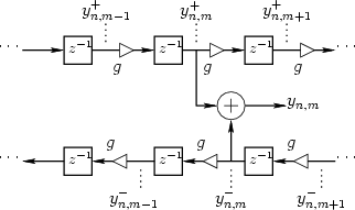
Figure G.7 depicts a digital waveguide section once again in ``physical canonical form,'' as shown earlier in Fig. G.5, and introduces a doubly indexed notation for greater clarity in the derivation below [420,207,116,115].

Figure G.7: Lossy digital waveguide--frequency-independent loss-factors $g$.

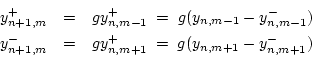
Referring to Fig. G.7, we have the following time-update relations:

$$\begin{eqnarray*} y^{+}_{n+1,m}&=& gy^{+}_{n,m-1}\;=\; g(y_{n,m-1}- y^{-}_{n,m-1... ...y^{-}_{n+1,m}&=& gy^{+}_{n,m+1}\;=\; g(y_{n,m+1}- y^{-}_{n,m+1}) \end{eqnarray*}$$

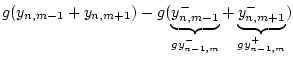
Adding these equations gives

$$y_{n+1,m} = g(y_{n,m-1}+y_{n,m+1}) - g(\underbrace{y^{-}_{n,m-1}}_{gy^{-}_{n-1,m}} + \underbrace{y^{-}_{n,m+1}}_{gy^{+}_{n-1,m}})$$

$$= g(y_{n,m-1}+y_{n,m+1}) - g^2 y_{n-1,m} \protect$$ (G.31)

This is now in the form of the finite-difference time-domain (FDTD) scheme analyzed in [207]:

$$y_{n+1,m}= g^{+}_my_{n,m-1}+ g^{-}_my_{n,m+1}+ a_my_{n-1,m},$$

with $g^{+}_m= g^{-}_m= g$, and $a_m= -g^2$. In [116], it was shown by von Neumann analysis (§L.4) that these parameter choices give rise to a stable finite-difference scheme (§L.2.3), provided $\vert g\vert\leq 1$. In the present context, we expect stability to follow naturally from starting with a passive digital waveguide model.