Von Neumann Analysis

Von Neumann analysis is used to verify the stability of a finite difference scheme (FDS). We will only consider FDSs having one time dimension, but any number of spatial dimensions.

The procedure, in principle, is to perform a spatial Fourier transform along all spatial dimensions, thereby reducing the FDS to a time recursion in terms of the spatial Fourier transform of the system. The system is then stable if this time recursion is at least marginally stable as a digital filter.

Let's apply von Neumann analysis to the FDS for the ideal vibrating string Eq.$\,$(M.3):

$$y_{n+1,m}= y_{n,m+1}+ y_{n,m-1}- y_{n-1,m} \protect$$

There is only one spatial dimension, so we only need a single 1D Discrete Time Fourier Transform (DTFT) along $m$ [456]. Using the shift theorem for the DTFT, we obtain

$$Y_{n+1}(k) = (e^{jkX} + e^{-jkX})Y_n(k) - Y_{n-1}(k)$$

$$= 2\cos(kX)Y_n(k) - Y_{n-1}(k)$$

$$\isdef 2c_kY_n(k) - Y_{n-1}(k) \protect$$ (M.8)

where $k=2\pi/\lambda$ denotes radian spatial frequency (wave number). (On a more elementary level, the DTFT along $m$ can be carried out by substituting $Y_n(k)e^{jkX}$ for $y(n,m)$ in the FDS.) This is now a second-order difference equation (digital filter) that needs its stability checked. This can be accomplished most easily using the Durbin recursion [455], or we can check that the poles of the recursion do not lie outside the unit circle in the $z$ plane.

A method equivalent to checking the pole radii, and typically used when the time recursion is first order, is to compute the amplification factor as the complex gain $G(k)$ in the relation

$$Y_{n+1}(k) = G(k)Y_n(k).$$

The FDS is then declared stable if $\vert G(k)\vert\leq 1$ for all spatial frequencies $k$.

Since the FDS of the ideal vibrating string is so simple, let's find the two poles. Taking the z transform of Eq.$\,$(M.8) yields

$$zY(z,k) = 2c_k Y(z,k) - z^{-1}Y(z,k)$$

yielding the following characteristic polynomial:

$$z^2 - 2c_k z - 1 = 0$$

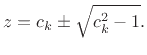
Applying the quadratic formula to find the roots yields

$$z = c_k \pm \sqrt{c_k^2 - 1}.$$

The squared pole moduli are then given by

$$\left\vert z\right\vert^2 = c_k^2 \pm (c_k^2 - 1) = \left\{\begi... ...eq 1 \\ [5pt] [1,1], & \left\vert c_k\right\vert\leq 1 \\ \end{array}\right..$$

Thus, for marginal stability, we require $\left\vert c_k\right\vert\leq 1$, and the poles become

$$z = c_k \pm j\sqrt{1-c_k^2} = \cos(kX) \pm j\sin(kX) = e^{\pm jkX}.$$

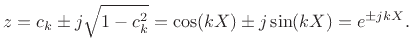
Since the range of spatial frequencies is $k\in[-\pi/X,\pi/X]$, we spontaneously have $\vert c_k\vert\leq1$ for all $k$. Therefore, we have shown by von Neumann analysis that the FDS Eq.$\,$(M.3) for the ideal vibrating string is stable.

In summary, von Neumann analysis verifies that no spatial Fourier components in the system are growing exponentially with respect to time.