Next |
Prev |
Up |
Top
|
Index |
JOS Index |
JOS Pubs |
JOS Home |
Search
The tone-hole reflectance and transmittance must be converted to
discrete-time form for implementation in a digital waveguide model.
Figure 9.49 plots the responses of second-order discrete-time
filters designed to approximate the continuous-time magnitude and phase
characteristics of the reflectances for closed and open toneholes, as
carried out in [406,409]. These filter designs
assumed a tonehole of radius  mm, minimum tonehole height
 mm, tonehole radius of curvature
 mm, and air column
radius
mm, and air column
radius  mm. Since the measurements of Keefe do not extend to 5
kHz, the continuous-time responses in the figures are extrapolated above
this limit. Correspondingly, the filter designs were weighted to produce
best results below 5 kHz.
mm. Since the measurements of Keefe do not extend to 5
kHz, the continuous-time responses in the figures are extrapolated above
this limit. Correspondingly, the filter designs were weighted to produce
best results below 5 kHz.
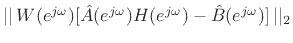
The closed-hole filter design was carried out using weighted
 equation-error minimization [432, p. 47], i.e., by minimizing
![$ \vert\vert\,W(\ejo)[{\hat A}(\ejo)H(\ejo) - {\hat B}(\ejo)]\,\vert\vert _2$](img2516.png) , where
, where  is the weighting
function,
is the weighting
function,  is the desired frequency response,
  denotes
discrete-time radian frequency, and the designed filter response is
denotes
discrete-time radian frequency, and the designed filter response is
 . Note that both phase and magnitude are
matched by equation-error minimization, and this error criterion is used
extensively in the field of system identification [290]
due to its ability to design optimal IIR filters via quadratic
minimization. In the spirit of the well-known Steiglitz-McBride algorithm
[289], equation-error minimization can be iterated,
setting the weighting function at iteration
. Note that both phase and magnitude are
matched by equation-error minimization, and this error criterion is used
extensively in the field of system identification [290]
due to its ability to design optimal IIR filters via quadratic
minimization. In the spirit of the well-known Steiglitz-McBride algorithm
[289], equation-error minimization can be iterated,
setting the weighting function at iteration  to the inverse of the
inherent weighting
to the inverse of the
inherent weighting
 of the previous iteration, i.e.,
 . However, for this study, the weighting was used only to
increase accuracy at low frequencies relative to high frequencies.
Weighted equation-error minimization is implemented in the matlab function
invfreqz() (§8.6.4).
. However, for this study, the weighting was used only to
increase accuracy at low frequencies relative to high frequencies.
Weighted equation-error minimization is implemented in the matlab function
invfreqz() (§8.6.4).
The open-hole discrete-time filter was designed using Kopec's method
[299], [432, p. 46] in conjunction with weighted equation-error
minimization. Kopec's method is based on linear prediction:
Use of linear prediction is equivalent to minimizing the
ratio error
This optimization criterion causes the filter to fit the upper
spectral envelope of the desired frequency-response. Since the first
step of Kopec's method captures the upper spectral envelope, the
``nulls'' and ``valleys'' are largely ``saved'' for the next step
which computes zeros. When computing the zeros, the spectral ``dips''
become ``peaks,'' thereby receiving more weight under the
ratio-error norm. Thus, in Kopec's method, the poles model the upper
spectral envelope, while the zeros model the lower spectral envelope.
To apply Kopec's method to the design of an open-tonehole filter, a
one-pole model
 was first fit to the continuous-time
response,
was first fit to the continuous-time
response,
 Subsequently, the inverse error spectrum,
 was modeled with a two-pole
digital filter,
was modeled with a two-pole
digital filter,
 The discrete-time approximation to
 was then given by

Figure 9.49:
Two-port
tonehole junction closed-hole and open-hole reflectances based on Keefe's
acoustic measurements (dashed) versus second-order digital filter
approximations (solid).
Top: Reflectance magnitude; Bottom: Reflectance
phase.
The closed tonehole has one resonance in the audio band just above  kHz.
The open tonehole has one anti-resonance in the audio band near
kHz.
The open tonehole has one anti-resonance in the audio band near  kHz.
At dc, the open tonehole fully reflects, while the closed tonehole reflects
close to nothing (from [406]).
kHz.
At dc, the open tonehole fully reflects, while the closed tonehole reflects
close to nothing (from [406]).
![\includegraphics[width=\twidth]{eps/twoptfilts}](img2534.png) |
The reasonably close match in both phase and magnitude by second-order
filters indicates that there is in fact only one important tonehole
resonance and/or anti-resonance within the audio band, and that the
measured frequency responses can be modeled with very high audio accuracy
using only second-order filters.
Figure 9.50 plots the reflection function calculated for a
six-hole flute bore, as described in [242].
Figure 9.50:
Reflection
functions for note  (three finger holes closed, three finger holes open) on a simple flute (from [406]). (top) Transmission-line calculation; (bottom) Digital waveguide two-port tonehole implementation.
![\includegraphics[width=\twidth]{eps/gtwoport}](img2535.png) |
The upper plot was calculated using Keefe's frequency-domain
transmission matrices, such that the reflection function was
determined as the inverse Fourier transform of the corresponding
reflection coefficient. This response is equivalent to that provided
by [242], though scale factor discrepancies exist due to
differences in open-end reflection models and lowpass filter
responses. The lower plot was calculated from a digital waveguide
model using two-port tonehole scattering junctions. Differences
between the continuous- and discrete-time results are most apparent in
early, high-frequency, closed-hole reflections. The continuous-time
reflection function was low-pass filtered to remove time-domain
aliasing effects incurred by the inverse Fourier transform operation
and to better correspond with the plots of [242]. By trial
and error, a lowpass filter with a cutoff frequency around 4 kHz was
found to produce the best match to Keefe's results. The digital
waveguide result was obtained at a sampling rate of 44.1 kHz and then
lowpass filtered to a 10 kHz bandwidth, corresponding to that of
[242]. Further lowpass filtering is inherent from the
first-order Lagrangian delay-line length interpolation technique used
in this model [506]. Because such filtering is applied at
different locations along the ``bore,'' a cumulative effect is
difficult to accurately determine. The first tonehole reflection is
affected by only two interpolation filters, while the second tonehole
reflection is affected by four of these filtering operations. This
effect is most responsible for the minor discrepancies apparent in the
plots.
Next |
Prev |
Up |
Top
|
Index |
JOS Index |
JOS Pubs |
JOS Home |
Search
[How to cite this work] [Order a printed hardcopy] [Comment on this page via email]
 .
.

