Frequency-Dependent Losses

The preceding derivation generalizes immediately to frequency-dependent losses. First imagine each $g$ in Fig.C.7 to be replaced by $G(z)$ , where for passivity we require

$$\left\vert G(e^{j\omega T})\right\vert\leq 1.$$

In the time domain, we interpret $g(n)$ as the impulse response corresponding to $G(z)$ . We may now derive the frequency-dependent counterpart of Eq.(C.31) as follows:

$$\begin{eqnarray*} y^{+}_{n+1,m}&=& g\ast y^{+}_{n,m-1}\;=\; g\ast (y_{n,m-1}- y^{-}_{n,m-1})\\ y^{-}_{n+1,m}&=& g\ast y^{-}_{n,m+1}\;=\; g\ast (y_{n,m+1}- y^{+}_{n,m+1})\\ [10pt] \Rightarrow\quad y_{n+1,m}&=& g\ast (y_{n,m-1}+y_{n,m+1}) - g\ast (\underbrace{y^{-}_{n,m-1}}_{g\ast y^{-}_{n-1,m}} + \underbrace{y^{+}_{n,m+1}}_{g\ast y^{+}_{n-1,m}})\nonumber \\ &=& g\ast (y_{n,m-1}+y_{n,m+1}) - g\ast g\ast y_{n-1,m}\\ &=& g\ast \left[(y_{n,m-1}+y_{n,m+1}) - g\ast y_{n-1,m}\right] \end{eqnarray*}$$

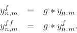
where $\ast$ denotes convolution (in the time dimension only). Define filtered node variables by

$$\begin{eqnarray*} y^f_{n,m}&=& g\ast y_{n,m}\\ y^{ff}_{n,m}&=& g\ast y^f_{n,m}. \end{eqnarray*}$$

Then the frequency-dependent FDTD scheme is simply

$$y_{n+1,m}= y^f_{n,m-1}+ y^f_{n,m+1}- y^{ff}_{n-1,m}.$$

We see that generalizing the FDTD scheme to frequency-dependent losses requires a simple filtering of each node variable 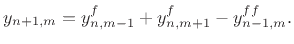$y_{n,m}$ by the per-sample propagation filter $G(z)$ . For computational efficiency, two spatial lines should be stored in memory at time $n$ : $y^f_{n,m}$ and $y^{ff}_{n-1,m}$ , for all $m$ . These state variables enable computation of $y_{n+1,m}$ , after which each sample of $y^f_{n,m}$ ($\forall m$ ) is filtered by $G(z)$ to produce $y^{ff}_{n-1,m}$ for the next iteration, and $y_{n+1,m}$ is filtered by $G(z)$ to produce $y^f_{n,m}$ for the next iteration.

The frequency-dependent generalization of the FDTD scheme described in this section extends readily to the digital waveguide mesh. See §C.14.5 for the outline of the derivation.