Next |
Prev |
Up |
Top
|
Index |
JOS Index |
JOS Pubs |
JOS Home |
Search
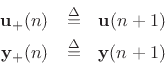
When
 in Eq.(2.10), the FDN (Fig.2.28)
reduces to a normal state-space model (§1.3.7),
in Eq.(2.10), the FDN (Fig.2.28)
reduces to a normal state-space model (§1.3.7),
The matrix
 is the state transition matrix.
The vector
is the state transition matrix.
The vector
![$ \mathbf{x}(n) = [x_1(n), x_2(n), x_3(n)]^T$](img546.png) holds the state
variables that determine the state of the system at time
holds the state
variables that determine the state of the system at time  . The
order of a state-space
system is equal to the number of state variables, i.e., the
dimensionality of
. The
order of a state-space
system is equal to the number of state variables, i.e., the
dimensionality of
 . The input and output signals have been
trivially redefined as
. The input and output signals have been
trivially redefined as
to follow normal convention for state-space form.
Thus, an FDN can be viewed as a generalized state-space model for a
class of  th-order linear systems--``generalized'' in the sense
that unit delays are replaced by arbitrary delays. This
correspondence is valuable for analysis because tools for state-space
analysis are well known and included in many software libraries such
as with matlab.
th-order linear systems--``generalized'' in the sense
that unit delays are replaced by arbitrary delays. This
correspondence is valuable for analysis because tools for state-space
analysis are well known and included in many software libraries such
as with matlab.
Next |
Prev |
Up |
Top
|
Index |
JOS Index |
JOS Pubs |
JOS Home |
Search
[How to cite this work] [Order a printed hardcopy] [Comment on this page via email]