 |
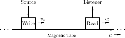
This analogy also works for a delay-line based computational model,
as depicted in Fig.5.5.
The magnetic tape is now the delay line, the tape read-head is the
read-pointer of the delay line, and the write-head is the delay-line
write-pointer. In this analogy, it is readily verified
that modulating delay by changing the read-pointer increment from 1 to
![]() (thereby requiring interpolated reads) corresponds to
listener motion toward the source at speed
(thereby requiring interpolated reads) corresponds to
listener motion toward the source at speed ![]() . It also follows
that changing the write-pointer increment from
. It also follows
that changing the write-pointer increment from ![]() to
to
![]() corresponds source motion away from the listener at
speed
corresponds source motion away from the listener at
speed ![]() .
When this is done, we must use interpolating writes into the
delay memory. Interpolating writes may be called
de-interpolation [506], and they are formally the
graph-theoretic transpose of interpolating reads (ordinary
``interpolation'') [336]. A review of
time-varying, interpolating, delay-line reads and writes, together
with a method using a single shared pointer, are given in
[386].
.
When this is done, we must use interpolating writes into the
delay memory. Interpolating writes may be called
de-interpolation [506], and they are formally the
graph-theoretic transpose of interpolating reads (ordinary
``interpolation'') [336]. A review of
time-varying, interpolating, delay-line reads and writes, together
with a method using a single shared pointer, are given in
[386].