State-Space BiQuad in FAUST

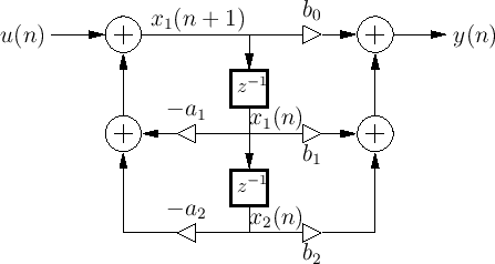
The block diagram of a general BiQuad filter section realized in Direct Form II is shown in Fig.21 [10].²⁷

Figure 21: Direct-Form-II implementation of a 2nd-order filter section, with state variables labeled as the delay outputs $x_1(n)$ and $x_2(n)$ .

From this diagram, we find the state-space matrices to be

$$A = \left[\begin{array}{cc} -a_1 & -a_2 \\ [2pt] 1 & 0 \end{array}\right] \qquad B = \left[\begin{array}{c} 1 \\ [2pt] 0 \end{array}\right] \qquad C = \left[\begin{array}{cc} b_1-b_0 a_1 & b_2-b_0 a_2 \end{array}\right] \qquad D = [\,b_0\,]$$

The FAUST code for the state-space realization of a specific resonator is shown in Fig.22.

Figure 22: FAUST state-space BiQuad filter, comparing to direct form.

 

// State-Space BiQuad Example

import("stdfaust.lib");

process = tpss; // state-space form
//process = tpdirect;   // direct form
//Test to compare outputs of the two:
//process = 1-1' <: tpdirect, tpss * (-1) :> _; // ~0

// Make direct-form coefficients for a simple resonator:
R = 0.9;         // pole radius
fc = ma.SR/10.0; // pole angle frequency in Hz
wcT = 2.0 * ma.PI * fc / ma.SR;
a1 = -2*R*cos(wcT);     a2 = R*R;
b0 = 1.0;       b1 = 0.0;       b2 = -1.0; // zeros at dc and SR/2

tpdirect = fi.tf2(b0,b1,b2,a1,a2); // filters.lib implementation

// State Space Model for Direct Form II:

p = 1; // number of inputs
q = 1; // number of outputs
N = 2; // number of states

a(1,1) = -a1;   a(1,2) = -a2;
a(2,1) = 1;     a(2,2) = 0;

b(1,1) = 1;
b(2,1) = 0;

c(1,1) = b1-b0*a1;      c(1,2) = b2-b0*a2;

d(1,1)= b0;

// We presently also need these catch-all rules (which are not used):
a(m,n) = 10*m+n;        b(m,n) = a(m,n);
c(m,n) = a(m,n);        d(m,n) = a(m,n);

matrix(M,N,f) = si.bus(N) <: ro.interleave(N,M) 
                : par(n,N, par(m,M,*(f(m+1,n+1)))) :> si.bus(M);

A = matrix(N,N,a);      B = matrix(N,p,b);
C = matrix(q,N,c);      D = matrix(q,p,d);

Bd = par(i,p,mem) : B; // input delay needed for conventional definition
vsum(N) = si.bus(2*N) :> si.bus(N); // vector sum of two N-vectors

tpss = si.bus(p) <: D, (Bd : vsum(N)~(A) : C) :> si.bus(q);