Next: Free End
Up: Boundary Conditions in the
Previous: Fixed End, Allowed to
Here the boundary conditions are
The boundary condition  is implemented as in the previous case. The condition
 requires some discussion.
Consider difference scheme (5.5) operating at the grid point  . By condition (5.13a),
  will be set to zero, so we do not need to use (5.5a) at all. The difference scheme used to update
  would be
if we had access to  , a value of the grid function
  at the grid location to the left of the boundary point. Since we don't, we eliminate it by use of the numerical boundary condition
which is a second-order accurate approximation to
. This leaves us with
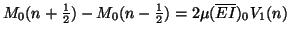 |
(5.15) |
Figure 5.4(b) shows the series junction terminated with a self-loop of impedance
 . We now show that with the proper setting of this impedance, this termination satisfies a numerical condition identical to (5.14). At this junction, there will only be two incoming waves,
 and
and
 , and we thus have:
Thus, by identification with (5.14), we require
and we can set
where the value of
 depends on the type of network we are using (see previous section). For a network of type II or III (see previous section),
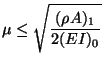
as defined above is automatically positive, if the stability conditions over the interior network junctions are satisfied, respectively (this is easily checked). For mesh of type I, we can show that it will be positive if it is true that
depends on the type of network we are using (see previous section). For a network of type II or III (see previous section),
as defined above is automatically positive, if the stability conditions over the interior network junctions are satisfied, respectively (this is easily checked). For mesh of type I, we can show that it will be positive if it is true that
Since, for a Type I network, we already must have condition (5.11) for stability over the problem interior, then assuming that the material parameters do not vary greatly from one grid point to the next (In the limit as
 , they must not), this boundary condition is stable for the type I mesh as well.
In this case it can be seen that one of the benefits of the waveguide formulation is that it is remarkably easy to check the compatibility of a particular type of boundary condition with a particular scheme. That is to say, the passivity condition, framed in terms of the positivity of the network immittances, even at the boundary, tells us immediately which boundary condition implementations will be stable. Compatibility can be checked directly in the finite difference framework, but the procedure (which form part of what is known as GKSO theory [176]) may be quite involved.
Next: Free End
Up: Boundary Conditions in the
Previous: Fixed End, Allowed to
Stefan Bilbao
2002-01-22