Next: Timoshenko's Beam Equations
Up: Boundary Conditions in the
Previous: Fixed Clamped End
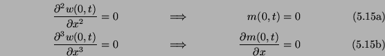
The boundary conditions are now
The condition  is the same as for the fixed end which is allowed to pivot. Thus we terminate the series junction in the same way as in that case. For the other condition,
 , there is complete symmetry with the case of the fixed clamped end, where the condition was
 . The junction can be terminated as in Figure 5.4(c), and we choose
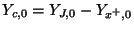 , where
 , and
, and
 follows from the particular type of mesh configuration that we are using. Stability of this boundary condition for the three types of mesh follows as before as well.
Figure 5.4:
Boundary terminations for the Euler-Bernoulli system-- (a) fixed end, allowed to pivot; (b) fixed, clamped end; (c) free end.
 |
Stefan Bilbao
2002-01-22