Finite Differences

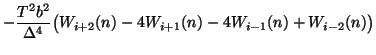
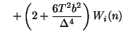
There are many ways to approach the numerical integration of (5.1). If the material parameters are constant, then a simple explicit method can be obtained by applying centered difference approximations to both the time and space derivatives, yielding the scheme

$$W_{i}(n+1)+W_{i}(n-1) = -\frac{T^{2} b^{2}}{\Delta^{4}}\big(W_{i+2}(n)-4W_{i+1}(n)-4W_{i-1}(n)+W_{i-2}(n)\big)\notag$$ (5.3)

$$\quad+\left(2+\frac{6T^{2}b^{2}}{\Delta^{4}}\right)W_{i}(n)$$ (5.4)

where $W_{i}(n)$ is a grid function defined for integer $i$ and $n$, and represents an approximation to $w(i\Delta,nT)$, where $\Delta$ is a uniform grid spacing, and $T$ is the time step. This scheme is accurate to $O(\Delta^{2},T^{2})$, but is stable only for $2b\frac{T}{\Delta^{2}}\leq 1$, so it is effectively only first-order accurate; this is typical of explicit methods for systems with some parabolic character [176].

In order to deal more effectively with the varying-coefficient problem, we can divide (5.1) into a system of two PDEs, and differentiate with respect to time, to get

$$\begin{eqnarray}\frac{\partial v}{\partial t} &=& -\frac{1}{\rho ... ...artial m}{\partial t} &=& EI\frac{\partial^{2}v}{\partial x^{2}} \end{eqnarray}$$ (5.5a)

Here, $v\triangleq \frac{\partial w}{\partial t}$ is the beam transverse velocity, and $m$ can be interpreted as a bending moment. We have chosen these variables in order to make clear the relationship of the classical beam theory with the more modern Timoshenko theory (see §5.2). Applying centered differences to this system yields

$$\begin{eqnarray}V_{i}(n+1)-V_{i}(n) &=& -\frac{\mu}{(\overline{\r... ...u(\overline{EI})_{i}\left(V_{i+1}(n)-2V_{i}(n)+V_{i-1}(n)\right) \end{eqnarray}$$ (5.6a)

where $V$ and $M$ are the grid functions corresponding to $v$ and $m$. Similarly to the case of the transmission line (see §4.3.6), we have used

$$(\overline{\rho A})_{i} = \rho(i\Delta)A(i\Delta)+O(\Delta^{2})$$

$$(\overline{EI})_{i} = E(i\Delta)I(i\Delta)+O(\Delta^{2})$$

and in keeping with the literature [176], we have also defined

$$\mu \triangleq \frac{T}{\Delta^{2}}$$

As for the transmission line, we can evaluate the grid functions $V$ and $M$ at alternating time steps. Due to the nature of the difference approximation, however, we cannot interleave these variables on the spatial grid. That is, we are forced to calculate both $V$ and $M$ at every grid location (at their respective time steps). We have written the difference scheme above such that temporal interleaving is evident, i.e. $V_{k}(m)$ and $M_{k}(m)$, $m$ half-integer, are calculated only for (say) $2m$ even and odd, respectively.