In (1+1)D, the hyperbolic system (4.17) requires two initial conditions. That is, we require the knowledge of initial current and voltage distributions along the line. We would like to enter the discrete equivalent of this data into the delay registers somehow at the first time step ![]() . From Figure 4.14, it should be clear that four sets of data are required:
. From Figure 4.14, it should be clear that four sets of data are required:
![]() ,
,
![]() ,
,
![]() , which are the initial incoming waves at the parallel junctions, and
, which are the initial incoming waves at the parallel junctions, and
![]() , the values initially stored in the self-loops at the series junctions.
, the values initially stored in the self-loops at the series junctions.
The first problem we encounter is that, on our decimated grid, we calculate values of ![]() and
and ![]() , the grid functions corresponding to voltage and current, at alternating time steps. We have chosen our grid such that for
, the grid functions corresponding to voltage and current, at alternating time steps. We have chosen our grid such that for ![]() and
and ![]() half-integer,
half-integer, ![]() is calculated for odd values of
is calculated for odd values of ![]() , and
, and ![]() for
for ![]() even; at time zero, then,
even; at time zero, then, ![]() is accessible (as a combination of wave variables). How then do we enter the current initial data into the algorithm? It turns out that this problem is rather simply addressed. We can do one of two things: set the value of
is accessible (as a combination of wave variables). How then do we enter the current initial data into the algorithm? It turns out that this problem is rather simply addressed. We can do one of two things: set the value of ![]() at time step
at time step
![]() to be equal to a sampled version of
to be equal to a sampled version of ![]() , and accept the error that this introduces, which will be
, and accept the error that this introduces, which will be ![]() , or we can use any available numerical method (i.e. one which does not operate on a staggered grid) to propagate the initial data
, or we can use any available numerical method (i.e. one which does not operate on a staggered grid) to propagate the initial data ![]() forward by
forward by ![]() . Such a method should be at least
. Such a method should be at least ![]() accurate, but it is allowed to even be unstable, since we will only be using it to update once [176].
accurate, but it is allowed to even be unstable, since we will only be using it to update once [176].
Assume then, that our initial data are
![]() , and
, and
![]() , some approximation to
, some approximation to
![]() obtained by either of the methods mentioned above. At time step
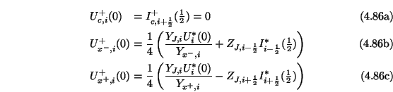
obtained by either of the methods mentioned above. At time step ![]() , we can write the junction voltages
, we can write the junction voltages
![]() as
as
We may ask, however, whether there is a way of setting the initial values such that we achieve better initial accuracy. For a network of type I, say, we have ![]() . Then, if
. Then, if
![]() is non-zero everywhere (this can always be arranged by operating slightly away from CFL), we may use
is non-zero everywhere (this can always be arranged by operating slightly away from CFL), we may use
These initialization procedures generalize simply to (2+1)D, where the parallel-plate equations require three initial conditions ![]() ,
,
![]() and
and
![]() . In general, we now have seven wave variables to set: the waves approaching any parallel junction with coordinates
. In general, we now have seven wave variables to set: the waves approaching any parallel junction with coordinates ![]() at
at ![]() , namely
, namely
![]() ,
,
![]() ,
,
![]() ,
,
![]() and
and
![]() , as well as the values stored in the self-loop registers at the series junctions,
, as well as the values stored in the self-loop registers at the series junctions,
![]() and
and
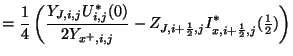
![]() . For the sake of brevity, we provide only the settings for the general case, analogous to (4.75):
. For the sake of brevity, we provide only the settings for the general case, analogous to (4.75):
 |
||||
 |
||||
 |
||||
 |
Because DWNs of the forms discussed in the previous sections are equivalent to two-step finite difference methods, problems with parasitic modes do not arise as they do in wave digital networks which simulate the same systems. This problem was discussed in detail in §3.9.