von Neumann Analysis

Frequency domain analysis of the scheme (6.33) is similar to that applied to the continuous time/space wave equation. As a shortcut to full $z$-transform, and spatial discrete Fourier transform analysis, consider again the behaviour of a test solution of the form

$$u_{i}^{n} = z^{n}e^{jl\beta h}$$ (6.37)

where $z = e^{nsk}$. This, again may be thought of as a wave-like solution, and in fact, it is identical to the wave-like solution employed in the continuous case, sampled at $t=nk$ and $x=lh$. When substituted into the difference scheme (6.34), the following characteristic equation results:

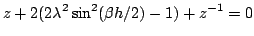$$z +2(2\lambda^2\sin^2(\beta h/2)-1)+z^{-1} = 0$$ (6.38)

which is analogous to (6.8). The roots are given by

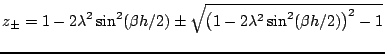$$z_{\pm} = 1-2\lambda^2\sin^2(\beta h/2)\pm\sqrt{\left(1-2\lambda^2\sin^2(\beta h/2)\right)^2-1}$$ (6.39)

Again, just as for the wave equation, there are two solutions (resulting from the fact that a second difference in time has been applied in scheme (6.33)), representing the propagation of the test solution in opposite directions.

One would expect that, in order for a solution such as (6.37) to behave as a solution to the wave equation, one should have $\vert z\vert=1$ for any value of $\beta$, the wavenumber--otherwise such a solution will experience exponential growth or damping. This is not necessarily true for scheme (6.33). From simple inspection of the characteristic equation (6.38), and using the same techniques applied to the harmonic oscillator in §, one may deduce that the roots are complex conjugates of unit magnitude when

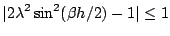$$\vert 2\lambda^2\sin^2(\beta h/2)-1\vert\leq 1$$ (6.40)

which can be rewritten as

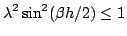$$\lambda^2\sin^2(\beta h/2)\leq 1$$ (6.41)

This inequality must be satisfied for any possible value of $\beta$. Because $\sin^2(\beta h/2)$ is bounded by one, the condition

$$\lambda\leq 1$$ (6.42)

is sufficient for stability. This is the famous Courant-Friedrichs-Lewy condition, which has the interesting physical interpretation as illustrated in Figure .

It is useful to note that for $\lambda$ slightly greater than unity, condition (6.41) will be violated near the maximum of the function $\sin^2(\beta h/2)$, which occurs at the wavenumber $\beta = \pi/h$, corresponding to a wavelength of $2h$--from basic sampling theory, this is the shortest wavelength which may be represented on a grid of spacing $h$. A typical result of numerical instability is then the explosive growth of such a component at the spatial Nyquist wavelength. See Figure 6.3.

Figure: Numerical Instability. Left to right: successive outputs $u$ of scheme (6.33), with a value of $\lambda = 1.0125$, violating condition (6.42). The sample rate and initial conditions are chosen as for the example shown in Figure 6.2. As time progresses, components of the solution near the spatial Nyquist frequency quickly grow in amplitude; within a few time steps after the last plot in this series, the computed values of the solution become out of range.