Numerical Dispersion

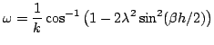
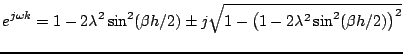
Consider now scheme (6.33) under the condition (6.42) that the roots of (6.38) are indeed of unit magnitude. These roots can be written, using $z=e^{j\omega k}$, as

$$e^{j\omega k} = 1-2\lambda^2\sin^2(\beta h/2)\pm j\sqrt{1-\left(1-2\lambda^2\sin^2(\beta h/2)\right)^2}$$ (6.43)

or

$$\omega = \frac{1}{k}\cos^{-1}\left(1-2\lambda^2\sin^2(\beta h/2)\right)$$ (6.44)

This is a dispersion relation for the scheme (6.33), relating frequency $\omega$ and wavenumber $\beta$ in complete analogy with the relation () for the wave equation itself.

Just as in the case of a continuous system, one may define a phase and group velocities for the scheme, now in a numerical sense, exactly as per (). In the case of the wave equation, recall that these velocities were constant, and equal to $\gamma$ for all wavenumbers. Now, however, both the phase and the group velocity are, in general, functions of wavenumber--in other words, different wavelengths travel at different speeds, and the scheme (6.33) is thus, in general, dispersive. This type of anomalous behaviour is purely a result of discretization, and is known as numerical dispersion--it should be carefully distinguished from physical dispersion of a model problem itself, which will appear when systems are subject to stiffness--such systems will be examined shortly in the next chapter. It is also clear that the numerical velocities will also depend on the choice of the parameter $\lambda$, which may be freely chosen for scheme (6.33), subject to the constraint (6.42). It is useful to plot the velocity curves, as functions of wavenumber for different values of $\lambda$, as shown in Figure .

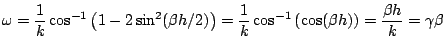
Now, consider the very special case of $\lambda = 1$. Under this condition, the dispersion relation (6.44) reduces to

$$\omega = \frac{1}{k}\cos^{-1}\left(1-2\sin^2(\beta h/2)\right) = \frac{1}{k}\cos^{-1}\left(\cos(\beta h)\right)=\frac{\beta h}{k} = \gamma\beta$$ (6.45)

Now, the numerical dispersion relation is exactly that of the continuous wave equation, and the phase and group velocities are both equal to $\gamma$, independently of $\beta$. There is thus no numerical dispersion for this choice of $\lambda$--this is another reflection of the fact that the scheme (6.33) is exact when $\lambda = 1$.

Figure: Numerical dispersion. Outputs for scheme (6.33) for the wave equation, at times as indicated, for $\lambda = 1$ (in grey) and $\lambda = 0.5$ (in black). $\gamma$ is chosen as 100, the sample rate is 16 000 Hz, and the initial conditions are set according to a narrow cosine distribution, of width 1/40. Notice that for $\lambda$ away from 1, the higher-frequency components in general lag the wavefront, illustrating the phase velocity characteristic of the scheme. Notice also that the gross speed of the wave packet is slower as well, illustrating the group velocity characteristic.