A Simple Finite Difference Scheme

The most rudimentary finite difference scheme for the 1D wave equation (and in almost all respects, the best) is given, in operator form, as

$$\delta_{tt}u = \gamma^2 \delta_{xx}u$$ (6.33)

Here, as mentioned previously, $u$ is shorthand notation for the grid function $u_{l}^{n}$, representing an approximation to the solution of the wave equation at $x=lh$, $t=nk$, where again, $h$ is the spacing between adjacent grid points, and $k$ is the time step. As the difference operators employed are second-order accurate, the scheme itself is in general, second order accurate in both time and space. (In fact, under a special choice of $h$ and $k$, its order of accuracy is infinite--in other words, it can yield an exact solution. This special case is confined to the simple wave equation alone, but forms the basis for digital waveguides, to be discussed in Section 6.2.9.)

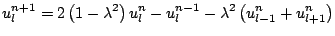
When the action of the operators is expanded out, a recursion results:

$$u_{l}^{n+1} = 2\left(1-\lambda^2\right)u_{l}^{n}-u_{l}^{n-1}-\lambda^2\left(u_{l-1}^n+u_{l+1}^n\right)$$ (6.34)

The important dimensionless parameter $\lambda$ has been defined here by

$$\lambda = \gamma k/h$$ (6.35)

This scheme may be updated, explicitly, at each time step $n$, from previously computed values at the previous two time steps. It is perhaps easiest to see the behaviour of this algorithm through a dependence plot showing the ''footprint" of the scheme (6.33), shown in Figure . For the sake of clarity, a typical output of the scheme (6.33) is presented here as well, in Figure 6.2.

For the moment, it is assumed that the spatial domain of the problem is infinite; the analysis of boundary conditions may thus be postponed temporarily, simplifying analysis somewhat.

Figure: Typical output of scheme (6.33). Left to right: successive outputs $u$ of scheme (6.33), at times as indicated, with a value of $\lambda = 1$. Here the sample rate is chosen as 8000 Hz, and $\gamma = 100$, and the initial conditions are chosen to correspond roughly to a pluck: both $u_{i}^{0}$ and $u_{i}^{1}$ have the form of raised cosine distributions, amplitude 1, and of spatial width 1/5.