Dispersion Relation

Frequency domain analysis is extremely revealing in the case of the wave equation in particular. Considering the case of a string defined over the spatial domain ${\mathcal D}={\mathbb{R}}$, a Fourier transform (in space) and a two-sided Laplace transform (in time) may be used. See Chapter 5 for more details. As a short-cut, one may analyze the behaviour of the test solution

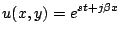$$u(x,y) = e^{st+j\beta x}$$ (6.6)

where $s$ is interpreted as a complex frequency variable, $s = \sigma + j\omega$, and $\beta$ is a real wavenumber. It is easy to see that if $\sigma = 0$, such a test solution is, in fact a traveling wave of temporal frequency $f = \omega/2\pi$, and wavelength $\lambda = 2\pi/\beta$. Substituting such a solution into (6.2) gives

$$(s^2+\gamma^2\beta^2)u = 0$$ (6.7)

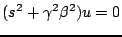
Clearly the test solution $u$ is non-zero everywhere, leading the characteristic equation

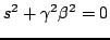$$s^2+\gamma^2\beta^2 = 0$$ (6.8)

which has roots

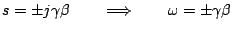$$s = \pm j\gamma\beta\qquad \Longrightarrow\qquad \omega = \pm \gamma\beta$$ (6.9)

This is known as the dispersion relation for the system (6.2); the frequency and wavenumber of a plane-wave solution are not independent. The fact that there are two solutions results from the fact that the wave equation is second order in time--the solutions correspond to left-going and right-going wave solutions.