The Delay Line

Figure 11: An example of a delay line and how it is used.

Figure 12: Equivalence between a vector of values and a delay line block diagram.

In this section we present the fundamental computing block used in physical modeling. We present different views of this data structure and use it for building string models for the remainder of this reader.

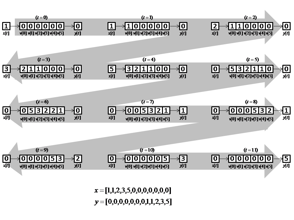
The data structure of the delay line naturally arose from digital computing. From a Computer Science perspective, the delay line is simply a vector of values. In the musical acoustics community, the delay line is the digital implementation of simulating propagation distance. Figure 11 shows an example of a length $6$ delay line, where at each time slice, values are shifted right. The input signal, into the delay line is $x(t)$ , such that the values input into the system are the first six non-zero numbers of the Fibonacci sequence.

As shown in Figure 11, the vector of values is used to represent space. At each tick, or change in time, the values shift right representing propagation of values. For the remainder of the reader, we assume that a delay line represents space and changes occur to its values through time. For simplification, we draw a delay line as a box with the negative exponent to the $z$ being the length of the delay. The $z$ corresponds to the variable of the $z$ -transform, where a single unit delay is $z^{-1}$ [2,3]. We denote this equivalence in Figure 12.

For the musical acoustics community, such a data structure is invaluable in modeling propagation. In reverberation, delay lines can be used to simulate the indirect paths of a signal [4,5]. Two online labs are available to help the reader gain familiarity with delay lines and how they are used in modeling propagation distance in a basic feed-forward block diagram and in more elaborate virtual reverberation algorithms. They can be found at http://ccrma.stanford.edu/realsimple/lattice_ladder/ and http://ccrma.stanford.edu/realsimple/reverb/, respectively.