Digital Waveguide Models

Figure 13: A digital waveguide consisting of two delay lines in series in a loop. Note that the inverters between the delay lines are only present when acceleration, velocity and displacement of the string is modeled.

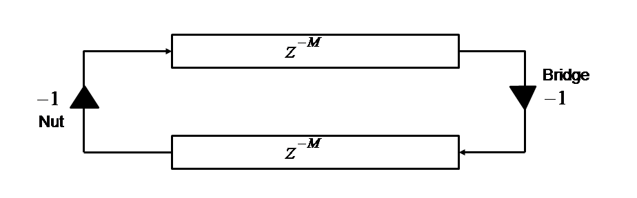
Observing the solution to the Wave Equation in Equation 2, the displacement of a string is the sum of two traveling waves moving in opposite directions. We model each traveling wave's propagation path with a delay line. As Figure 13 shows, the data-structure of two delay lines in series in a loop models the physical behavior of the vibrating string as the virtual implementation of the theoretical solution of the sum of two traveling waves.

To cement these abstractions, we present an example of how a vibrating string is modeled with the digital waveguide with initial conditions of a triangular pulse near the middle of the string. Since the sum of the left and right traveling-wave components always equals the displacement of the physical string, we initialize each delay line with a triangular pulse with half the amplitude of the physical string such that the sum of corresponding values from both delay lines equals the amplitude of the pluck for the physical string.

At $t=0$ , we allow values to propagate. Depending on what the sampling-rate is, the physical length of each sample in the delay lines is set assuming a constant propagation speed $c$ .

As Figures 3 to 10 show, the string is held in place at points $P1$ , $P2$ and $P3$ . At $t=0$ , we release the string at these points. What we obtain from our virtual model is two traveling waves moving in opposite directions such that the sum of corresponding values always equals the displacement of the physical string [6].

We now relate the parameters of the digital waveguide to physical characteristics of the string. Our simple digital waveguide, shown in Figure 13, consists of two delay lines each of length $M$ . The frequency of the digital waveguide is directly related to the sampling-rate of our system and the length of the delay lines, $M$ .

Assuming a sampling rate $f_s$ , we can determine how long it would take for an impulse to travel to both ends of the string and back. If an impulse is placed in the first sample of the first delay line, we confirm that it takes $2M$ samples of propagation for the impulse to return to its original position, which is equivalent to $T = \frac{2M}{f_s}$ seconds. Therefore, in our lossless string-model, a traveling-wave takes $T$ seconds to reflect from one end and back. Inverting $T$ , we now know that the virtual string oscillates at a fundamental of $f_1 = \frac{1}{T}$ Hz.

Since each delay line corresponds to one direction of a traveling wave of the string, we have an intuitive physical mapping between the digital waveguide and the physical string. In Figure 13, we have inverters between the two delay lines. The inverter on the left of the figure corresponds to the ``nut'' of the instrument and the second inverter the ``bridge'' of the instrument. Note that the inverters are only present in our digital waveguide when acceleration, velocity and displacement waves are modeled with the waveguide. For a more detailed discussion on alternative wave variables modeled in digital waveguides, we refer readers to http://ccrma.stanford.edu/~jos/pasp/Alternative_Wave_Variables.html.