 |
|
|
The formulation of the Wave Equation and its solution by d'Alembert in 1747 [1] is the theoretical starting-point for physical stringed models. The wave equation, written as
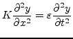 |
(1) |
where ![]() is the string tension,
is the string tension,
![]() is the linear mass density and
is the linear mass density and ![]() is the string
displacement as a function of time (
is the string
displacement as a function of time (![]() ) and position along the string (
) and position along the string (![]() ).
It can be derived directly from Newton's second law applied to a differential
string element. In addition to introducing the 1D wave equation, d'Alembert
introduced its solution in terms of traveling waves:
).
It can be derived directly from Newton's second law applied to a differential
string element. In addition to introducing the 1D wave equation, d'Alembert
introduced its solution in terms of traveling waves:
where
![]() denotes the wave propagation speed.
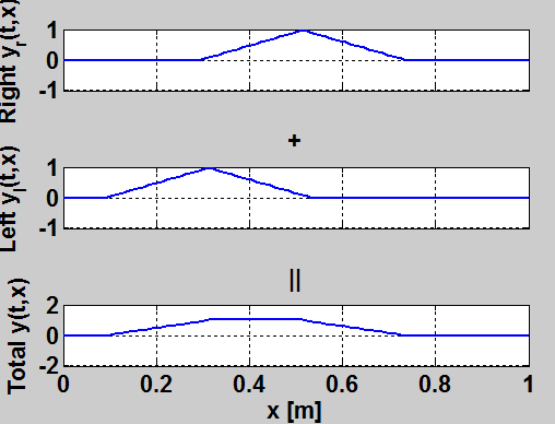
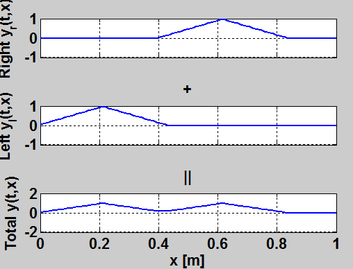
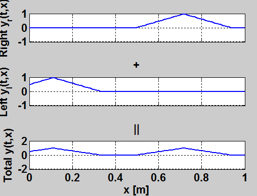
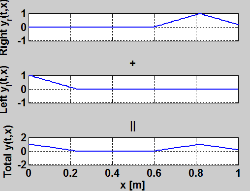
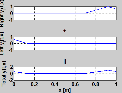
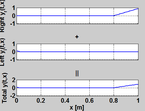
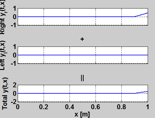
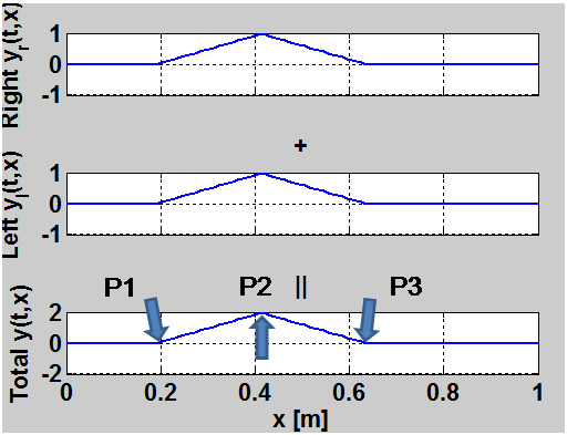
Though each individual traveling wave is unobservable in the physical world, we use their constructs for modeling
the physical behavior of the string, whose displacement is equal to the sum of the
two traveling waves. Figures 3 to 10 show how a physical string's displacement,
initially displaced to a triangular pulse, is equal to the sum of its left and right traveling waves at time
denotes the wave propagation speed.
Though each individual traveling wave is unobservable in the physical world, we use their constructs for modeling
the physical behavior of the string, whose displacement is equal to the sum of the
two traveling waves. Figures 3 to 10 show how a physical string's displacement,
initially displaced to a triangular pulse, is equal to the sum of its left and right traveling waves at time ![]() .
The blue arrows in Figure 3 show the points of displacement at time
.
The blue arrows in Figure 3 show the points of displacement at time ![]() . Subsequent frames
are shown, as the bottom plot of each frame corresponds to the physical displacement of the string. The top and bottom
plots correspond to the right and left traveling waves, respectively. For a detailed derivation of
the solution to the Wave Equation, we refer readers to
. Subsequent frames
are shown, as the bottom plot of each frame corresponds to the physical displacement of the string. The top and bottom
plots correspond to the right and left traveling waves, respectively. For a detailed derivation of
the solution to the Wave Equation, we refer readers to
http://ccrma.stanford.edu/~jos/pasp/Traveling_Wave_Solution_I.html.
D'Alembert's solution to the wave equation serves as the theoretical foundation of which physical models for stringed instruments are based upon.