 ), as
shown in the right portion of the figure. The channel signals
), as
shown in the right portion of the figure. The channel signals
We now turn to various practical examples of perfect reconstruction filter banks, with emphasis on those using FFTs in their implementation (i.e., various STFT filter banks).
Figure 11.28 illustrates a generic filter bank with ![]() channels,
much like we derived in §9.3.
The analysis filters
channels,
much like we derived in §9.3.
The analysis filters ![]() ,
,
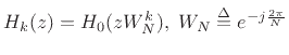
![]() are bandpass filters
derived from a lowpass prototype
are bandpass filters
derived from a lowpass prototype ![]() by modulation (e.g.,
), as
shown in the right portion of the figure. The channel signals
by modulation (e.g.,
), as
shown in the right portion of the figure. The channel signals
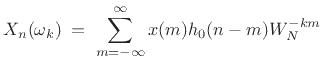
![]() are given by the convolution of the input signal with
the
are given by the convolution of the input signal with
the ![]() th channel impulse response:
th channel impulse response:
Suppose the analysis window ![]() (flip of the baseband-filter impulse
response
(flip of the baseband-filter impulse
response ![]() ) is length
) is length ![]() . Then in the context of overlap-add
processors (Chapter 8),
. Then in the context of overlap-add
processors (Chapter 8), ![]() is a Portnoff
window, and implementing the window with a length
is a Portnoff
window, and implementing the window with a length ![]() FFT requires
that the windowed data frame be time-aliased down to length
FFT requires
that the windowed data frame be time-aliased down to length
![]() prior to taking a length
prior to taking a length ![]() FFT (see §9.7). We can
obtain this same result via polyphase analysis, as elaborated in the
next section.
FFT (see §9.7). We can
obtain this same result via polyphase analysis, as elaborated in the
next section.
![\begin{psfrags}
% latex2html id marker 30995\psfrag{z^-1}{{\large $z^{-1}$}}\psfrag{X(z)}{{\large $X(z)$}}\psfrag{X0(z)}{{\large $X_0(z)$}}\psfrag{X1(z)}{{\large $X_1(z)$}}\psfrag{X2(z)}{{\large $X_2(z)$}}\psfrag{Xn[0]}{{\normalsize $X_n(\omega_0)$}}\psfrag{Xn[1]}{{\normalsize $X_n(\omega_1)$}}\psfrag{Xn[2]}{{\normalsize $X_n(\omega_2)$}}\psfrag{H0(z)}{{\large $H_0(z)$}}\psfrag{H1(z)}{{\large $H_1(z)$}}\psfrag{H2(z)}{{\large $H_2(z)$}}\psfrag{W(-0n,N)}{{\small $W_N^{0n}$}}\psfrag{W(-1n,N)}{{\small $W_N^{-1n}$}}\psfrag{W(-2n,N)}{{\small $W_N^{-2n}$}}\psfrag{W(0n,N)}{{\small $W_N^{0n}$}}\psfrag{W(1n,N)}{{\small $W_N^{1n}$}}\psfrag{W(2n,N)}{{\small $W_N^{2n}$}}\psfrag{STFT}{}\begin{figure}[htbp]
\includegraphics[width=\twidth]{eps/portnoff}
\caption{Portnoff analysis bank for $N=3$.}
\end{figure}
\end{psfrags}](img2225.png)