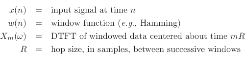
Overlap-Add (OLA) STFT Processing

This chapter discusses use of the Short-Time Fourier Transform (STFT) to implement linear filtering in the frequency domain. Due to the speed of FFT convolution, the STFT provides the most efficient single-CPU implementation engine for most FIR filters encountered in audio signal processing.

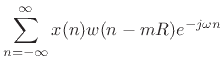
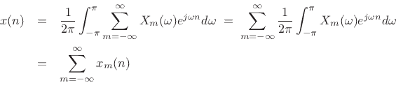
Recall from §7.1 the STFT:

$$X_m(\omega) = \sum_{n=-\infty}^{\infty} x(n) w(n-mR) e^{-j\omega n}$$

$$= \hbox{\sc DTFT}_\omega(x\cdot\hbox{\sc Shift}_{mR}(w)) \protect$$ (9.1)

where

$$\begin{eqnarray*} x(n) &=& \hbox{input signal at time $n$}\\ w(n) &=& \hbox{window function (\textit{e.g.}, Hamming)}\\ X_m(\omega) &=& \hbox{DTFT of windowed data centered about time $mR$}\\ R &=& \hbox{hop size, in samples, between successive windows}\\ \end{eqnarray*}$$

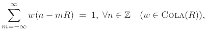
We noted that if the window $w(n)$ has the constant overlap-add property at hop-size $R$ ,

$$\sum_{m=-\infty}^{\infty} w(n-mR) \eqsp 1, \;\forall n\in\mathbb{Z} \quad \hbox{($w\in\hbox{\sc Cola}(R)$)},$$ (9.2)

then the sum of the successive DTFTs over time equals the DTFT of the whole signal $X(\omega)$ :

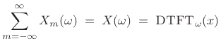$$\sum_{m=-\infty}^\infty X_m(\omega) \eqsp X(\omega) \eqsp \hbox{\sc DTFT}_\omega(x)$$ (9.3)

Consequently, the inverse-STFT is simply the inverse-DTFT of this sum:

$$\begin{eqnarray*} x(n) &=& \frac{1}{2\pi}\int_{-\pi}^\pi \sum_{m=-\infty}^\infty X_m(\omega) e^{j\omega n} d\omega \eqsp \sum_{m=-\infty}^\infty \frac{1}{2\pi}\int_{-\pi}^\pi X_m(\omega) e^{j\omega n} d\omega\\ &=& \sum_{m=-\infty}^\infty x_m(n) \end{eqnarray*}$$

We may now introduce spectral modifications by multiplying each spectral frame $X_m(\omega)$ by some filter frequency response $H_m(\omega)$ to get

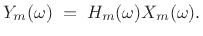$$Y_m(\omega) \eqsp H_m(\omega)X_m(\omega).$$ (9.4)

Note that $H_m$ can be different for each frame, giving a certain class of time-varying filters. The filtered output signal spectrum is then

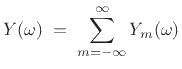$$Y(\omega) \eqsp \sum_{m=-\infty}^\infty Y_m(\omega)$$ (9.5)

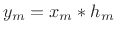
so that

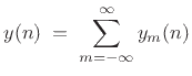$$y(n) \eqsp \sum_{m=-\infty}^\infty y_m(n)$$ (9.6)

where

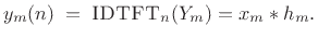$$y_m(n) \eqsp \hbox{\sc IDTFT}_n(Y_m) = x_m\ast h_m.$$ (9.7)

This chapter discusses practical implementation of the above relations using a Fast Fourier Transform (FFT). In particular, we use an FFT to compute efficiently what may be regarded as a sampled DTFT. We will look at how sampling density must be increased along the unit circle when spectral modifications are to be performed, and we will discuss further the COLA condition on the analysis window and hop-size. In the end, our practical FFT-convolution engine will look as follows:

$$y \eqsp \sum_{m=-\infty}^\infty \hbox{\sc Shift}_{mR} \left( \hbox{\sc FFT}_N^{-1} \left\{ H_m \cdot \hbox{\sc FFT}_N\left[\hbox{\sc Shift}_{-mR}(x)\cdot w_M \right]\right\}\right)$$ (9.8)

The sum over $m$ may be interpreted as adding separately filtered frames $y_m=x_m\ast h_m$ . Due to this filtering, the frames must overlap, even when the rectangular window is used. As a result, the overall system is often called an overlap-add FFT processor, or ``OLA processor'' for short. It is regarded as a sequence of FFTs which may be modified, inverse-transformed, and summed. This ``hopping transform'' view of the STFT is the Fourier dual of the ``filter-bank'' interpretation to be discussed in Chapter 9.