Effect of Windowing

Let's look at a simple example of windowing to demonstrate what happens when we turn an infinite-duration signal into a finite-duration signal through windowing.

We begin with a sampled complex sinusoid:

$$s_{\omega_0}(n) = e^{j \omega_0 n T }, \quad n \in \mathbb{Z}$$ (6.14)

A portion of the real part, $\cos(\omega_0 nT)$ , is plotted in Fig.5.3. The imaginary part, $\sin(\omega_0 nT)$ , is of course identical but for a 90-degree phase-shift to the right.

Figure: A portion of the real part of the sinusoid $s_{\omega _0}(n)$ .

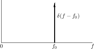
The Fourier transform of this infinite-duration signal is a delta function at $\omega=\omega_0$ . I.e., $S_{\omega_0}(\omega) = 2\pi\delta(\omega-\omega_0) = \delta(f-f_0)$ , as indicated in Fig.5.4.

Figure: Spectrum (DTFT) of an infinite-duration sinusoid at frequency $f_0$ Hz.

The windowed signal is

$$s_R(n) = w(n)e^{j \omega_0 n T}, \quad n \in \mathbb{Z}$$ (6.15)

as shown in Fig.5.5. (Note carefully the difference between $w$ and $\omega$ .)

Figure 5.5: Windowed sinusoid real part.

The convolution theorem (§2.3.5) tells us that our multiplication in the time domain results in a convolution in the frequency domain. Hence, we will obtain the convolution of $\delta(\omega-\omega_0)$ with the Fourier transform of the window $W(\omega)$ . This is easy since the delta function is the identity element under convolution ( $\delta \ast W = W$ ). However, since our delta function is at frequency $\omega=\omega_0$ , the convolution shifts the window transform out to that frequency:

$$S_R(\omega) = W(\omega)\ast 2\pi\delta(\omega - \omega_0) = 2\pi W(\omega-\omega_0)$$ (6.16)

This is shown in Fig.5.6.

Figure 5.6: Fourier transform of the windowed sinusoid in Fig.5.5: Top: Real Fourier transform amplitude. Bottom: Fourier transform magnitude in decibels (dB).

From comparing Fig.5.6 with the ideal sinusoidal spectrum in Fig.5.4 (an impulse at frequency $\omega_0$ ), we can make some observations:

• Windowing in the time domain resulted in a ``smearing'' or ``smoothing'' in the frequency domain. In particular, the infinitely thin delta function has been replaced by the ``main lobe'' of the window transform. We need to be aware of this if we are trying to resolve sinusoids which are close together in frequency.

• Windowing also introduced side lobes. This is important when we are trying to resolve low amplitude sinusoids in the presence of higher amplitude signals.

• A sinusoid at amplitude $A$ , frequency $\omega_0$ , and phase $\phi$ manifests (in practical spectrum analysis) as a window transform shifted out to frequency $\omega_0$ , and scaled by $A e^{j\phi}$ .

As a result of the last point above, the ideal window transform is an impulse in the frequency domain. Since this cannot be achieved in practice, we try to find spectrum-analysis windows which approximate this ideal in some optimal sense. In particular, we want side-lobes that are as close to zero as possible, and we want the main lobe to be as tall and narrow as possible. (Since absolute scalings are normally arbitrary in signal processing, ``tall'' can be defined as the ratio of main-lobe amplitude to side-lobe amplitude--or main-lobe energy to side-lobe energy, etc.) There are many alternative formulations for ``approximating an impulse'', and each such formulation leads to a particular spectrum-analysis window which is optimal in that sense. In addition to these windows, there are many more which arise in other applications. Many commonly used window types are summarized in Chapter 3.