Traveling waves in continuous media are discussed in Appendix G. However, we will summarize the main facts here. While this section is concerned with applying scattering theory to lumped modeling, it is clearest to derive the basic scattering relations in the traveling wave case.
In a traveling wave, force is in phase with velocity. For left-going waves on a string, the minus sign takes care of the fact that a given force (which is proportional to string slope) acts to the left and right with opposite signs. For waves in an acoustic tube, the minus sign properly accounts for longitudinal velocity waves in each direction.
The ratio of force to velocity in a traveling wave, ![]() above, is called
the wave impedance. When the wave impedance changes, from
above, is called
the wave impedance. When the wave impedance changes, from ![]() to
to
![]() , say, scattering occurs at a junction connecting the
two impedances, i.e., the traveling wave splits into reflected and
transmitted components. This follows immediately from the basic
traveling-wave relations above and from physical continuity.
, say, scattering occurs at a junction connecting the
two impedances, i.e., the traveling wave splits into reflected and
transmitted components. This follows immediately from the basic
traveling-wave relations above and from physical continuity.
In vibrating strings, the wave impedance is given by
![]() where
where
![]() is the string tension and
is the string tension and ![]() is mass density. Thus, one way to
change the wave impedance along a stretched string is to change the string
density by adjoining two strings of different material or thickness. It is
more difficult to change the string tension since a ``frictionless vertical
guide rod'' is necessary, in principle. At a junction between two wave
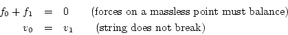
impedances on a string, the physical continuity constraints are that
velocity is unchanged across the junction (to avoid breaking the string)
and the net vertical force at the junction, obtained by summing the force
applied by each string endpoint at the junction, must be zero (to avoid
accelerating a zero mass at the junction). Therefore, the junction is
formally a series connection of the two ports representing the
string endpoints which are joined.
is mass density. Thus, one way to
change the wave impedance along a stretched string is to change the string
density by adjoining two strings of different material or thickness. It is
more difficult to change the string tension since a ``frictionless vertical
guide rod'' is necessary, in principle. At a junction between two wave
impedances on a string, the physical continuity constraints are that
velocity is unchanged across the junction (to avoid breaking the string)
and the net vertical force at the junction, obtained by summing the force
applied by each string endpoint at the junction, must be zero (to avoid
accelerating a zero mass at the junction). Therefore, the junction is
formally a series connection of the two ports representing the
string endpoints which are joined.
In acoustic tubes, the wave impedance is given by ![]() where
where
![]() is the cross-sectional area of the tube (and the velocity variable
is volume velocity). Thus, the easy way to introduce a
scattering junction in an acoustic tube is to change the
cross-sectional area discontinuously. This is why the vocal
tract is modeled as a piecewise cylindrical acoustic tube in speech
modeling [275,82]. At an area discontinuity in an acoustic
tube, the physical continuity constraints are that the pressure must
be continuous across the junction (to avoid accelerating a massless
plane of air at the junction), and the volume velocities (which are
taken as positive when flowing into the junction) must sum to zero at
the junction (so that air particles are not created or destroyed).
Thus, in acoustic tubes, parallel junctions naturally arise
between sections of two different wave impedance.
is the cross-sectional area of the tube (and the velocity variable
is volume velocity). Thus, the easy way to introduce a
scattering junction in an acoustic tube is to change the
cross-sectional area discontinuously. This is why the vocal
tract is modeled as a piecewise cylindrical acoustic tube in speech
modeling [275,82]. At an area discontinuity in an acoustic
tube, the physical continuity constraints are that the pressure must
be continuous across the junction (to avoid accelerating a massless
plane of air at the junction), and the volume velocities (which are
taken as positive when flowing into the junction) must sum to zero at
the junction (so that air particles are not created or destroyed).
Thus, in acoustic tubes, parallel junctions naturally arise
between sections of two different wave impedance.
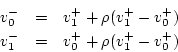
It is quick to derive the scattering relations for either the ideal string
or acoustic tube. Let
![]() denote the traveling force wave
components immediately to the left of a junction in a string, and let
denote the traveling force wave
components immediately to the left of a junction in a string, and let
![]() denote the components on the right, as shown in
Fig. J.12. Similarly define the velocity wave components. The
physical continuity constraints can be written
denote the components on the right, as shown in
Fig. J.12. Similarly define the velocity wave components. The
physical continuity constraints can be written
![\includegraphics[scale=0.9]{eps/lstringscat}](img2560.png) |
Let ![]() denote the common velocity of the string endpoints meeting at
a junction. (All velocities are taken as positive in the upward direction.)
Then since
denote the common velocity of the string endpoints meeting at
a junction. (All velocities are taken as positive in the upward direction.)
Then since
![]() , continuity implies
, continuity implies
![]() .
Therefore, we have
.
Therefore, we have
A scattering diagram is shown in Fig. J.13.
This is the so-called Kelly-Lochbaum form [275]. However, it is important to notice that the scattering equations can also be written
which is diagrammed in Fig. J.14.
Thus, a scattering junction fundamentally requires only one multiplication and three additions.
![\includegraphics[scale=0.9]{eps/lscat_vel_series}](img2572.png)
![\includegraphics[scale=0.9]{eps/lscatVelSeriesOneMul}](img2574.png)