Feedback Comb Filter Amplitude Response

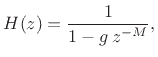
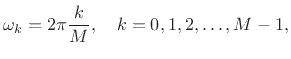
Figure 2.26 shows a family of feedback-comb-filter amplitude responses, obtained using a selection of feedback coefficients.

Figure 2.26: Amplitude response of the feedback comb-filter $H(z) = 1/(1-g z^{-M})$ (Fig.2.24 with $b_0=1$ and $-a_M=g$ ) with $M=5$ and $g=0.1$ , $0.5$ , and $0.9$ . a) Linear amplitude scale. b) Decibel scale.

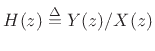
Figure 2.27 shows a similar family obtained using negated feedback coefficients; the opposite sign of the feedback exchanges the peaks and valleys in the amplitude response.

Figure 2.27: Amplitude response of the phase-inverted feedback comb-filter, i.e., as in Fig.2.26 with negated $g=-0.1$ , $-0.5$ , and $-0.9$ . a) Linear amplitude scale. b) Decibel scale.

As introduced in §2.6.2 above, a class of feedback comb filters can be defined as any difference equation of the form

$$y(n) = x(n) + g\,y(n-M).$$

Taking the z transform of both sides and solving for $H(z)\isdef Y(z)/X(z)$ , the transfer function of the feedback comb filter is found to be

$$H(z) = \frac{1}{1-g\,z^{-M}}, \protect$$ (3.5)

so that the amplitude response is

$$G(\omega) \isdef \left\vert H(\ejo)\right\vert = \frac{1}{\left\vert 1 - g e^{-j\omega M}\right\vert}, \quad -\pi \leq \omega \leq \pi .$$

This is plotted in Fig.2.26 for $M=5$ and $g=0.1$ , $0.5$ , and $0.9$ . Figure 2.27 shows the same case but with the feedback sign-inverted.

For $g=1$ , the feedback-comb amplitude response reduces to

$$G(\omega) = \frac{1}{2\left\vert\sin(\omega M/2)\right\vert},$$

and for $g=-1$ to

$$G(\omega) = \frac{1}{2\left\vert\cos(\omega M/2)\right\vert},$$

which exactly inverts the amplitude response of the feedforward comb filter with gain $g=1$ (Eq.(2.4)).

Note that $g>0$ produces resonant peaks at

$$\omega_k = 2\pi\frac{k}{M}, \quad k=0,1,2,\dots,M-1,$$

while for $g<0$ , the peaks occur midway between these values.