The ideal transformer, depicted in Fig. C.39 a, is a
lossless two-port electric circuit element which scales up voltage by
a constant ![]() [110,35]. In other words, the voltage at
port 2 is always
[110,35]. In other words, the voltage at
port 2 is always ![]() times the voltage at port 1. Since power is
voltage times current, the current at port 2 must be
times the voltage at port 1. Since power is
voltage times current, the current at port 2 must be ![]() times the
current at port 1 in order for the transformer to be lossless. The
scaling constant
times the
current at port 1 in order for the transformer to be lossless. The
scaling constant ![]() is called the turns ratio because
transformers are built by coiling wire around two sides of a
magnetically permeable torus, and the number of winds around the port
2 side divided by the winding count on the port 1 side gives the
voltage stepping constant
is called the turns ratio because
transformers are built by coiling wire around two sides of a
magnetically permeable torus, and the number of winds around the port
2 side divided by the winding count on the port 1 side gives the
voltage stepping constant ![]() .
.
![\includegraphics[width=\twidth]{eps/lTransformer}](img4173.png) |
In the case of mechanical circuits, the two-port transformer relations appear as
![\begin{eqnarray*}
F_2(s) &=& g F_1(s) \\ [5pt]
V_2(s) &=& \frac{1}{g} V_1(s)
\end{eqnarray*}](img4174.png)
where ![]() and
and ![]() denote force and velocity, respectively.
We now convert these transformer describing
equations to the wave variable formulation. Let
denote force and velocity, respectively.
We now convert these transformer describing
equations to the wave variable formulation. Let ![]() and
and ![]() denote
the wave impedances on the port 1 and port 2 sides,
respectively, and define velocity as positive into the transformer. Then
denote
the wave impedances on the port 1 and port 2 sides,
respectively, and define velocity as positive into the transformer. Then

Similarly,
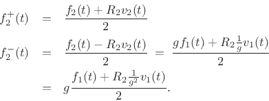
We see that choosing

eliminates the scattering terms and gives the simple relations
![\begin{eqnarray*}
f^{{-}}_2(t) &=& g f^{{+}}_1(t)\\ [5pt]
f^{{-}}_1(t) &=& \frac{1}{g}f^{{+}}_2(t).
\end{eqnarray*}](img4178.png)
The corresponding wave flow diagram is shown in Fig. C.39 b.
Thus, a transformer with a voltage gain ![]() corresponds to simply
changing the wave impedance from
corresponds to simply
changing the wave impedance from ![]() to
to ![]() , where
, where
![]() . Note that the transformer implements a change
in wave impedance without scattering as occurs in physical
impedance steps (§C.8).
. Note that the transformer implements a change
in wave impedance without scattering as occurs in physical
impedance steps (§C.8).