Wave Digital Dashpot

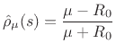
Starting with a dashpot with coefficient $\mu$ , we have

$$R(s) = \mu$$   (Dashpot Impedance)

and reflectance

$$\hat{\rho}_\mu(s) = \frac{\mu - R_0 }{\mu + R_0}$$

This time, choosing $R_0$ equal to the element value gives

$$\hat{\rho}_\mu(s) = 0$$

Conformally mapping the zero function yields the zero function so that

$$\fbox{$\displaystyle \hat{\tilde{\rho}}_\mu(z) = 0$} \qquad\mbox{(Wave Digital Dashpot)}$$

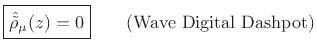
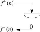
as well. Thus, the WDF of a dashpot is a ``wave sink,'' as diagrammed in Fig.F.4.

Figure F.4: Wave flow diagram for the Wave Digital Dashpot.

In the context of waveguide theory, a zero reflectance corresponds to a matched impedance, i.e., the terminating transmission-line impedance equals the characteristic impedance of the line.

The difference equation for the wave digital dashpot is simply $f^{{-}}(n)=0$ . While this may appear overly degenerate at first, remember that the interface to the element is a port at impedance $R_0=\mu$ . Thus, in this particular case only, the infinitesimal waveguide interface is the element itself.