Plane Wave Sampling Theory

This section develops a special case of Wave Field Synthesis (WFS) by spatially sampling simple plane waves. Sampling plane waves is much simpler than the traditional WFS formulation which begins with the classical Kirchhoff-Helmholtz integral (Firtha, 2018; Pierce, 1989). In return for this simplicity, we are restricted to virtual primary sources that are many wavelengths away from the speaker array, and on the other side of it from the listener. As we shall see, we can relax these restrictions in various ways, and the remaining sampling conditions are generally equally binding for WFS systems. In other words, spatial sampling theory is fundamental to all spatial audio systems using discrete drivers arranged in linear, planar, or even more general array geometries. What does not seem to be generally known, however, is that a sampling-based approach is sufficient (and much more to the point) for deriving and optimizing the system, as pursued in this paper.

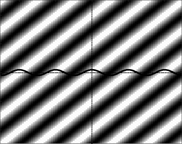
Figure 2 shows a monochromatic plane wave traveling down and to the right at a 45 degree angle. The solid black line across the middle represents the microphone-array, ideally a uniformly spaced grid of tiny omnidirectional pressure microphones having no ``acoustic shadow'' at all; these microphones serve to sample the plane wave along the line. In the 3D case, the line represents one cut along a planar microphone-array. The sinusoid drawn along the microphone line indicates the pressure seen by each microphone. 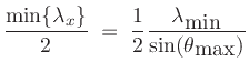By the sampling theorem (applied now to spatial sampling using a microphone-array), we must have more than two microphones per wavelength $\lambda_x$ along the line array. Thus, the required microphone density is determined by the minimum incident wavelength $\lambda_{\mbox{min}}$ and the maximum angle of incidence $\theta_{\mbox{max}}$ , as derived below.

Figure 2: Cross-section of a single-frequency plane wave traveling down and to the right into a line-array of microphones.

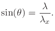
Figure 3 illustrates the geometry of the wavelengths involved. The wavelength of the incident sinusoidal plane wave is denoted $\lambda$ , and $\lambda_x$ denotes the wavelength of the sinusoidal pressure fluctuation seen by the microphone line array. As Fig.3 makes clear, from the angle of incidence $\theta$ and incident wavelength $\lambda$ , we have

$$\sin(\theta) = \frac{\lambda }{\lambda_x }.$$ (1)

Let $\Delta_x$ denote the microphone spacing along the $x$ axis. Then the sampling theorem requires

$$\Delta_x < \frac{\min\{\lambda_x \}}{2} \eqsp \frac{1}{2}\frac{\lambda_{\mbox{min}}}{\sin(\theta_{\mbox{max}})}$$ (2)

$$= \frac{c}{2\cdot f_{\mbox{max}}\cdot\sin(\theta_{\mbox{max}})}$$ (3)

where $c$ is the speed of sound (m/s), $f_{\mbox{max}}$ is the maximum temporal frequency in Hz (typically 20 kHz for audio), and $\theta_{\mbox{max}}$ (radians) is the maximum plane-wave angle allowed.

Figure 3: Wavelength geometry.

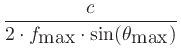
For example, choosing $f_{\mbox{max}}= 19.5$ kHz and $\theta_{\mbox{max}}=\pi/4$ (stage angle 90 degrees), and using $c=343$ m/s for sound speed, we obtain $\Delta_x <12.5$ mm, or about half-inch spacing for the microphones. (The coincident speaker-array has the same sampling-density requirement as the microphone-array.)

Reducing either $f_{\mbox{max}}$ or $\theta_{\mbox{max}}$ relaxes the spatial sampling density requirement. For example, if the ``stage width'' is reduced from 90 degrees ( $\theta_{\mbox{max}}=\pi/4\approx0.8$ ) down to 40 degrees ( $\theta_{\mbox{max}} = \pi\cdot 20/180 \approx 0.35$ ), then one-inch spacing of the microphones (and speakers) is allowed. If we band-limit our reconstruction bandwidth to 5 kHz, then we get by with four-inch spacing, as pursued below in a practical PBAP design (§2.15).

If we don't band-limit to below the spatial Nyquist limit, then we obtain ``spatial angle aliasing'' at very high frequencies for sources near the left or right edge of the ``stage viewing window''. That is, for sources near the left or right edges of the ``stage'', the highest-frequency components may not appear to come from the same direction as components below the cutoff frequency of 5 kHz. On the other hand, perception is such that the apparent angle-of-arrival typically may not alias at high frequencies because the desired angle remains a psychoacoustic choice and keeps the whole source spectrum in one place. Sources near the center of the stage are spatially oversampled by the microphone-array at all frequencies, so they are never a problem. In lowpassed-wideband-noise tests (see Appendix A), high-frequency spatial aliasing has been observed to break up a formerly coherent wideband virtual noise source, but not in a manner indicating ``folding'' as in aliasing of tones due to temporal sampling, but instead as the sound of a spurious new noise source somewhere along the array. The psychoacoustics of spatial aliasing perception is a fascinating topic for ongoing research.