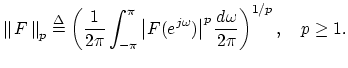
The ![]() norms are defined on the space
norms are defined on the space ![]() by
by
Since all practical desired frequency responses arising in digital
filter design problems are bounded on the unit circle, it follows that
![]() forms a Banach space under any
forms a Banach space under any ![]() norm.
norm.
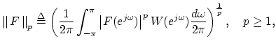
The weighted ![]() norms are defined by
norms are defined by
The case ![]() gives the popular root mean square norm, and
gives the popular root mean square norm, and
![]() can be interpreted as the total energy of
can be interpreted as the total energy of
![]() in many physical contexts.
in many physical contexts.
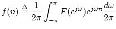
An advantage of working in ![]() is that the norm is provided by an
inner product,
is that the norm is provided by an
inner product,

As ![]() approaches infinity in Eq. (1), the error measure is dominated
by the largest values of
approaches infinity in Eq. (1), the error measure is dominated
by the largest values of
![]() . Accordingly, it is customary to
define
. Accordingly, it is customary to
define
Suppose the ![]() norm of
norm of
![]() is finite, and let
is finite, and let
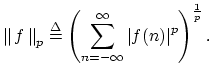
The norms for impulse response sequences
![]() are defined in a
manner exactly analogous with the frequency response norms
are defined in a
manner exactly analogous with the frequency response norms
![]() ,
viz.,
,
viz.,
The ![]() and
and ![]() norms are strictly concave functionals for
norms are strictly concave functionals for
![]() (see below).
(see below).
By Parseval's theorem, we have
![]() , i.e., the
, i.e., the ![]() and
and ![]() norms are the same for
norms are the same for ![]() .
.
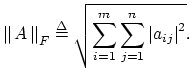
The Frobenious norm of an ![]() matrix
matrix ![]() is defined as
is defined as
Theorem. The unique ![]() rank
rank ![]() matrix
matrix ![]() which minimizes
which minimizes
![]() is given by
is given by
![]() , where
, where
![]() is a singular value decomposition of
is a singular value decomposition of ![]() , and
, and ![]() is formed
from
is formed
from ![]() by setting to zero all but the
by setting to zero all but the ![]() largest singular
values.
largest singular
values.
Proof. See Golub and Kahan [3].
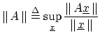
The induced norm of a matrix ![]() is defined in terms of the norm defined
for the vectors
is defined in terms of the norm defined
for the vectors
![]() on which it operates,
on which it operates,

The Hankel matrix corresponding to a time series ![]() is defined by
is defined by
![]() , i.e.,
, i.e.,
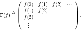
The Hankel norm of a filter frequency response is defined as the spectral norm of the Hankel matrix of its impulse response,
If ![]() is strictly stable, then
is strictly stable, then
![]() is finite for all
is finite for all
![]() , and all norms defined thus far are finite. Also, the Hankel
matrix
, and all norms defined thus far are finite. Also, the Hankel
matrix ![]() is a bounded linear operator in this case.
is a bounded linear operator in this case.
The Hankel norm is bounded below by the ![]() norm, and bounded above
by the
norm, and bounded above
by the
![]() norm [1],
norm [1],