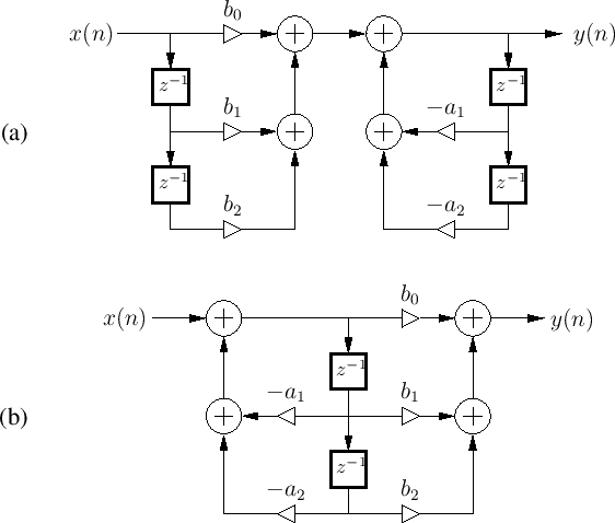
One possible signal flow graph (or system diagram)
for Eq.(5.1) is given in
Fig.5.1a for the case of ![]() and
and ![]() .
Hopefully, it is easy to see how this diagram represents the
difference equation (a box labeled ``
.
Hopefully, it is easy to see how this diagram represents the
difference equation (a box labeled ``![]() '' denotes a one-sample
delay in time). The diagram remains true if it is converted to the
frequency domain by replacing all time-domain signals by their
respective z transforms (or Fourier transforms); that is, we may replace
'' denotes a one-sample
delay in time). The diagram remains true if it is converted to the
frequency domain by replacing all time-domain signals by their
respective z transforms (or Fourier transforms); that is, we may replace
![]() by
by ![]() and
and ![]() by
by ![]() .
. ![]() transforms and their usage
will be discussed in Chapter 6.
transforms and their usage
will be discussed in Chapter 6.
 |