Next |
Prev |
Up |
Top
|
Index |
JOS Index |
JOS Pubs |
JOS Home |
Search
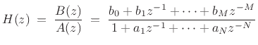
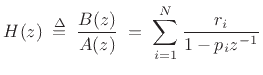
In summary, the partial fraction expansion can be used to expand
any rational z transform
as a sum of first-order terms
 |
(7.17) |
for  , and
, and
 |
(7.18) |
for  , where the term
 is optional, but often
preferred. For real filters, the complex one-pole terms may be paired
up to obtain second-order terms with real coefficients.
The PFE procedure occurs in two or three steps:
is optional, but often
preferred. For real filters, the complex one-pole terms may be paired
up to obtain second-order terms with real coefficients.
The PFE procedure occurs in two or three steps:
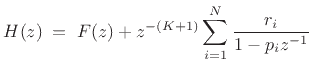
- When
, perform a step of long division to obtain
an FIR part
 and a strictly proper IIR part
 .
.
- Find the
 poles
poles  ,
,
 (roots of
  ).
).
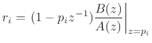
- If the poles are distinct, find the
coefficients (residues)
 ,
from
,
from
- If there are repeated poles, find the additional coefficients via
the method of §6.8.5, and the general form of the PFE is
 |
(7.19) |
where  denotes the number of distinct poles, and
 denotes the multiplicity of the
  th pole.
In step 2, the poles are typically found by factoring the
denominator polynomial
. This is a dangerous step numerically
which may fail when there are many poles, especially when many poles
are clustered close together in the  plane.
The following matlab code illustrates factoring
 to
obtain the three roots,
to
obtain the three roots,
 ,
,  :
:
A = [1 0 0 -1];  % Filter denominator polynomial
poles = roots(A) % Filter poles
See Chapter 9 for additional discussion regarding digital filters
implemented as parallel sections (especially §9.2.2).
Next |
Prev |
Up |
Top
|
Index |
JOS Index |
JOS Pubs |
JOS Home |
Search
[How to cite this work] [Order a printed hardcopy] [Comment on this page via email]