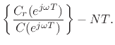
The definition of group delay,
does not give an immediately useful recipe for computing group delay numerically. In this section, we describe the theory of operation behind the matlab function for group-delay computation given in §J.8.
A more useful form of the group delay arises from the
logarithmic derivative of the frequency response. Expressing
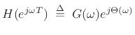
the frequency response
![]() in polar form as
in polar form as
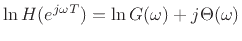
yields the following logarithmic decomposition of magnitude and phase:
Thus, the real part of the logarithm of the frequency response equals the log amplitude response, while the imaginary part equals the phase response.
Since differentiation is linear, the logarithmic derivative becomes

where
 im
im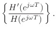 im
im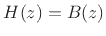
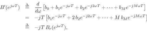
Consider first the FIR case in which
![\begin{eqnarray*}
B^\prime(e^{j\omega T}) &\isdef & \frac{d}{d\omega}\left[b_0
+ b_1 e^{-j\omega T}
+ b_2 e^{-j2\omega T}
+ \cdots
+ b_M e^{-jM\omega T}\right]\\
&=& -jT\left[b_1 e^{-j\omega T}
+ 2\, b_2 e^{-j2\omega T}
+ \cdots
+ M\,b_M e^{-jM\omega T}\right]\\
&\isdef & -jT\,B_r(e^{j\omega T}),
\end{eqnarray*}](img947.png)
where ![]() denotes ``
denotes ``![]() ramped'', i.e., the
ramped'', i.e., the ![]() th coefficient of
the polynomial
th coefficient of
the polynomial ![]() is
is ![]() , for
, for
![]() . In
matlab, we may compute Br from B via the
following statement:
. In
matlab, we may compute Br from B via the
following statement:
Br = B .* [0:M]; % Compute ramped B polynomialThe group delay of an FIR filter
 im
im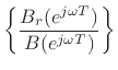 re
re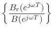
In matlab, the group delay, in samples, can be computed simply as
D = real(fft(Br) ./ fft(B))where the fft, of course, approximates the Discrete Time Fourier Transform (DTFT). Such sampling of the frequency axis by this approximation is information-preserving whenever the number of samples (FFT length) exceeds the polynomial order
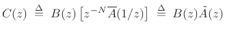
Finally, when there are both poles and zeros, we have
where

may be called the ``flip-conjugate'' or ``Hermitian conjugate'' of the polynomial
C = conv(B,fliplr(conj(A)));It is straightforward to show (Problem 11) that
The phase of the IIR filter
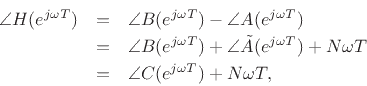
and the group delay computation thus reduces to the FIR case:
 re
re
This method is implemented in §J.8.

![$\displaystyle C(z) \isdefs B(z)\left[ z^{-N}\overline{A}(1/z)\right] \isdefs B(z)\tilde{A}(z) \protect$](img961.png)