In any real vibrating string, there are energy losses due to yielding
terminations, drag by the surrounding air, and internal friction within the
string. While losses in solids generally vary in a complicated way with
frequency, they can usually be well approximated by a small number of
odd-order terms added to the wave equation. In the simplest case, force is
directly proportional to transverse string velocity, independent of
frequency. If this proportionality constant is ![]() , we obtain the
modified wave equation
, we obtain the
modified wave equation
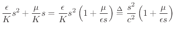
Setting
![]() in the wave equation to find the relationship
between temporal and spatial frequencies in the eigensolution, the wave
equation becomes
in the wave equation to find the relationship
between temporal and spatial frequencies in the eigensolution, the wave
equation becomes
 |
|||
 |
 is the wave velocity in the lossless case.
At high frequencies (large
is the wave velocity in the lossless case.
At high frequencies (large  |
(C.22) |
 |
(C.23) |
![$\displaystyle e^{st+vx} = \exp{\left[st\pm \left({s + \frac{\mu}{2\epsilon }}\right)\frac{x}{c}\right]} = \exp{\left[s\left(t\pm \frac{x}{c}\right)\right]} \exp{\left(\pm\frac{\mu}{2\epsilon }\frac{x}{c}\right)}.$](img3339.png) |
(C.24) |
| (C.25) |
| (C.26) |
Setting ![]() and using superposition to build up arbitrary traveling
wave shapes, we obtain the general class of solutions
and using superposition to build up arbitrary traveling
wave shapes, we obtain the general class of solutions
| (C.27) |
Sampling these exponentially decaying traveling waves at intervals of
![]() seconds (or
seconds (or ![]() meters) gives
meters) gives
![\begin{eqnarray*}
y(t_n,x_m) &=& e^{-{\left(\mu/2\epsilon \right)}{x_m/c}} y_r\left(t_n-{x_m/c}\right)
+ e^{{\left(\mu/2\epsilon \right)}{x_m/c}} y_l\left(t_n+{x_m/c}\right)\\
&=& e^{-{\left(\mu/2\epsilon \right)}{mX/c}} y_r\left(nT-{mX/c}\right)
+ e^{{\left(\mu/2\epsilon \right)}{mX/c}} y_l\left(nT+{mX/c}\right)\\
&=& e^{-{\mu mT/2\epsilon }} y_r\left[(n-m)T\right]
+ e^{ {\mu mT/2\epsilon }} y_l\left[(n+m)T\right]\\
&=& \left(e^{-{\mu T/2\epsilon }}\right)^m y^{+}(n-m)
+ \left(e^{ {\mu T/2\epsilon }}\right)^m y^{-}(n+m) \\
&\isdef & g^{m} y^{+}(n-m) + g^{-m} y^{-}(n+m).
\end{eqnarray*}](img3343.png)
The simulation diagram for the lossy digital waveguide is shown in Fig.C.5.
Again the discrete-time simulation of the decaying traveling-wave solution
is an exact implementation of the continuous-time solution at the
sampling positions and instants, even though losses are admitted in the
wave equation. Note also that the losses which are distributed in
the continuous solution have been consolidated, or lumped, at
discrete intervals of ![]() meters in the simulation. The loss factor
meters in the simulation. The loss factor
![]() summarizes the distributed loss incurred in one
sampling interval. The lumping of distributed losses does not introduce
an approximation error at the sampling points. Furthermore, bandlimited
interpolation can yield arbitrarily accurate reconstruction between
samples. The only restriction is again that all initial conditions and
excitations be bandlimited to below half the sampling rate.
summarizes the distributed loss incurred in one
sampling interval. The lumping of distributed losses does not introduce
an approximation error at the sampling points. Furthermore, bandlimited
interpolation can yield arbitrarily accurate reconstruction between
samples. The only restriction is again that all initial conditions and
excitations be bandlimited to below half the sampling rate.
![\includegraphics[scale=0.9]{eps/floss}](img3344.png)