Next |
Prev |
Up |
Top
|
JOS Index |
JOS Pubs |
JOS Home |
Search
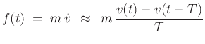
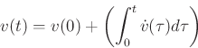
The velocity  can be written as
In particular,
- This approximation replaces a one-sample integral
by the area under the trapezoid having vertices
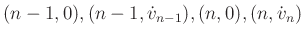
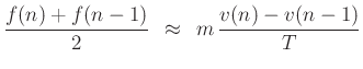
- In other words,
 is
approximated by a straight line between time
is
approximated by a straight line between time  and
and 
- This is a first-order approximation of
in contrast to
the zero-order approximation used by forward and backward Euler
schemes
- We will see that the commonly used bilinear transform is equivalent
- Model is exact if driving force is piecewise linear, having a constant slope over each sampling interval
- (Backward Euler is similarly exact for a piecewise-constant driving force)
Bilinear Transform as Compensated BE/FE
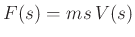
In Newton's law  , look at the Backward Euler (BE)
approximation of the time-derivative:
, look at the Backward Euler (BE)
approximation of the time-derivative:
We see there is a 1/2 sample delay in the first-order difference on
the right. This misaligns the force  and subsequent velocity by
half a sample. A very simple delay compensation is to use a
two-point average on the left:
and subsequent velocity by
half a sample. A very simple delay compensation is to use a
two-point average on the left:
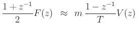
The extra attenuation at high frequencies due to the two-point average
actually helps. Taking the  transform:
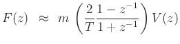
or
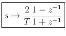
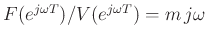
which is the bilinear transform of
 :
:
Frequency Warping is the Only Error
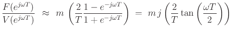
We have
using the bilinear transform (trapezoidal integration in the time domain)
Let's look along the unit circle in the
plane:
Since the exact formula is
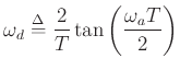
 , we can push all of the error
into a frequency warping:
, we can push all of the error
into a frequency warping:
- Frequency-warping is the only error over the unit circle when using the bilinear transform
- What started out as different gain errors on the left and right became the
correct gains at warped frequency locations
- Frequency-warping implications should also be considered in the time domain
Next |
Prev |
Up |
Top
|
JOS Index |
JOS Pubs |
JOS Home |
Search
Download DigitizingNewton.pdf
Download DigitizingNewton_2up.pdf
Download DigitizingNewton_4up.pdf
![\begin{eqnarray*}
v(nT) % &=& v(0) + \int_{0}^{nT}\vt(\tau)d\tau \\ [10pt]
&=& v(0) + \int_{0}^{(n-1)T}\dot v(\tau)d\tau + \int_{(n-1)T}^{nT}\dot v(\tau)d\tau \\ [10pt]
&=& v[(n-1)T]+\int_{(n-1)T}^{nT}\dot v(\tau)d\tau \\ [10pt]
&\approx& v[(n-1)T] +T\frac{\dot v[(n-1)T] + \dot v(nT)}{2}
\end{eqnarray*}](img85.png)