 |
As discussed in Section 2.1.4, the loop filter
gives the Digital Waveguide frequency-dependent damping. Similar to what
is used in Artificial Reverbation, the time for frequencies to decay
![]() dB, known as
dB, known as ![]() , is used to determine the gains of the filter.
We define
, is used to determine the gains of the filter.
We define ![]() to be the time in seconds for a signal to decay
to be the time in seconds for a signal to decay
![]() dB. For obtaining gains for the fundamental and harmonics of our
loop filter, we compute
dB. For obtaining gains for the fundamental and harmonics of our
loop filter, we compute ![]() for each of these frequencies over time
using the Energy Decay Relief (EDR) [36,41].
for each of these frequencies over time
using the Energy Decay Relief (EDR) [36,41].
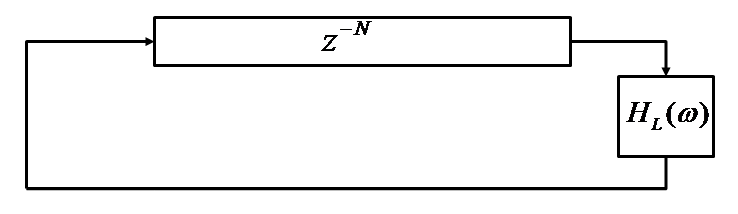
For the remainder of this section, we commute the second delay line shown in Figure 14 with the loop filter and combine the delay lines. The resulting system, shown in Figure 29 is equivalent to the one shown in Figure 14 as the delay line and loop filter components are linear and time-invariant.
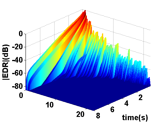
Similar to the STFT, the EDR shows the spectral components over time of a given signal. The single difference between the STFT and the EDR is that the square magnitudes of the FFT of each frame is used instead of the magnitudes. With the EDR, the amount of energy in each FFT bin is given over time. An advantage of using the EDR over the STFT is that energy decreases monotonically, whereas magnitudes, as used by the STFT, may increase and decrease resulting in noisier data for decay estimation.
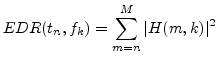
The EDR is defined as follows
 |
(9) |
where ![]() corresponds to the
corresponds to the ![]() th FFT bin at frame
th FFT bin at frame ![]() of the EDR.
of the EDR. ![]() corresponds to the total number of frames in our EDR. Thus,
corresponds to the total number of frames in our EDR. Thus,
![]() represents the total amount of energy remaining in the signal at
time
represents the total amount of energy remaining in the signal at
time ![]() for frequency
for frequency ![]() . Figure 30
shows a three-dimensional plot of the EDR over time and frequency.
. Figure 30
shows a three-dimensional plot of the EDR over time and frequency.
Since the displacement of the string decreases exponentially, viewing its motion and EDR in log space, we expect linear decays, as Figure 30 shows for a plucked guitar string note.
 |
 |
 |
 |
 |
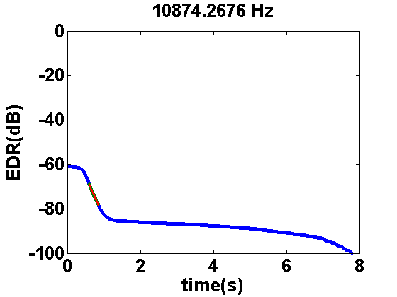 |
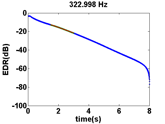
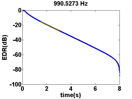
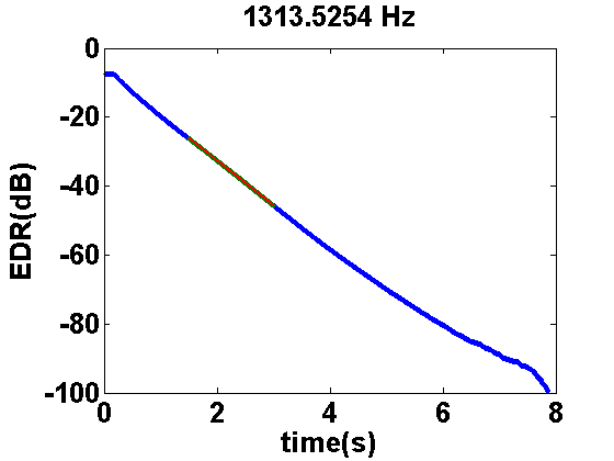
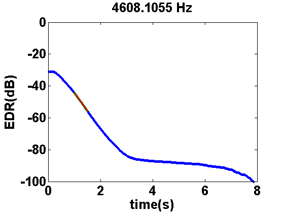
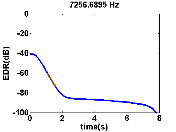
For each frequency ![]() in the set of frequencies closest to the fundamental and harmonic
frequencies, we fit a line to the time-decay of its EDR. The primary
parameter for estimation is the slope of the line. Figures 31 to 36 show EDR plots for
the fundamental frequency and five harmonics. The EDR for each frequency over time is plotted in blue.
The estimated line is shown in red. The estimation used only the segments of the EDR for which the red line
overlaps the blue. As shown, the line estimated nearly matches exactly the subset of EDR points used.
in the set of frequencies closest to the fundamental and harmonic
frequencies, we fit a line to the time-decay of its EDR. The primary
parameter for estimation is the slope of the line. Figures 31 to 36 show EDR plots for
the fundamental frequency and five harmonics. The EDR for each frequency over time is plotted in blue.
The estimated line is shown in red. The estimation used only the segments of the EDR for which the red line
overlaps the blue. As shown, the line estimated nearly matches exactly the subset of EDR points used.
Given the estimated slope, ![]() , for frequency
, for frequency ![]() ,
,
![]() . With
. With ![]() computed
for the fundamental and harmonic frequencies, we now relate the decay times to the gains of the loop filter.
computed
for the fundamental and harmonic frequencies, we now relate the decay times to the gains of the loop filter.
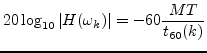
where
![]() corresponds to the per sample desired gain of our filter. We also have the relation that
corresponds to the per sample desired gain of our filter. We also have the relation that
| (11) |
| (12) |
where
![]() is the desired loop filter gain. This relates our per sample gain with the desired
loop filter gain in series with a length
is the desired loop filter gain. This relates our per sample gain with the desired
loop filter gain in series with a length ![]() delay line.
Substituting
delay line.
Substituting
![]() for
for
![]() in Equation 10, we obtain
in Equation 10, we obtain
| (13) |
Taking
![]() of both sides yields
of both sides yields
 |
(14) |
To specify gains at frequencies between the fundamental and harmonics, we linearly interpolate between points for which we have gains for. In specials cases, the gains at DC up until the fundamental frequency are set to the value of the gain computed at the fundamental. For frequencies between the last harmonic and half the sampling-rate, the gains decrease at an arbitrary slope.
With the gains specified for the loop filter, a complex spectrum with minimum-phase is computed [42]. A least-squares fit or the Steiglitz-McBride iteration is used to compute the coefficients for an arbitrary order filter [42,43].
 |
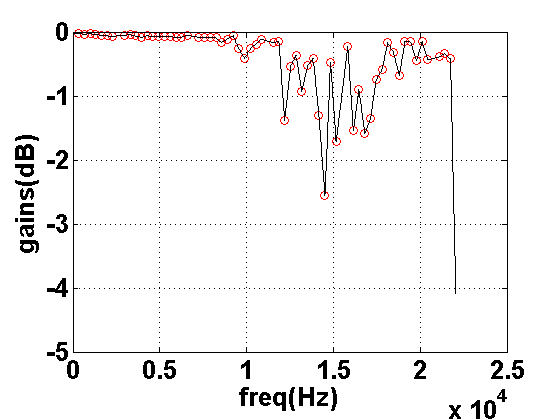 |
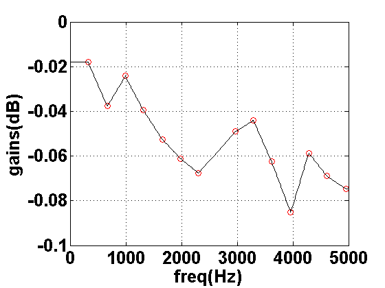
Figures 37 and 38 show the desired gains computed for a recorded guitar note. The fundamental is ![]() Hz.
Gains for the fundamental and harmonic frequencies are circled in red. All other
points are linearly interpolated between these gains and the constants we set for DC and half the sampling-rate.
Gains below the fundamental to DC are
set to the value of the gain at the fundamental frequency.
The gain at half the sampling-rate was arbitrarily set to
Hz.
Gains for the fundamental and harmonic frequencies are circled in red. All other
points are linearly interpolated between these gains and the constants we set for DC and half the sampling-rate.
Gains below the fundamental to DC are
set to the value of the gain at the fundamental frequency.
The gain at half the sampling-rate was arbitrarily set to ![]() dB.
Figure 37 shows gains from DC up to
dB.
Figure 37 shows gains from DC up to ![]() kHz.
kHz.