 |
 |
 |
 |
As discussed in Section 2.2, the excitation to our virtual instrument is a signal, taken from a wave-table used to drive our digital waveguide models. In the literature there are several methods for computing excitation signals from actual recordings. Extracting excitations from actual recordings of guitar plucks result in the best, psychoacoustically sounding models [33].
In recent years, two fundamentally different approaches for obtaining excitation signals from recordings have emerged: inverse-filtering and constant overlap-add (COLA) methods. We briefly describe the problem and give an overview of the various methods.
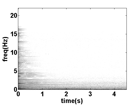
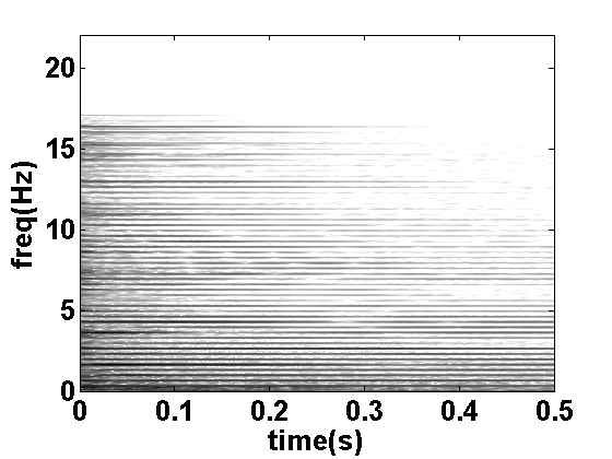
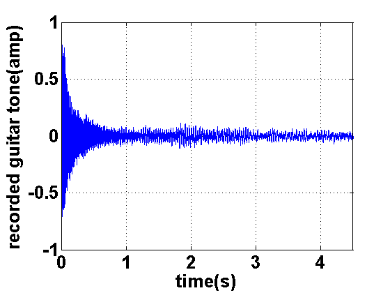
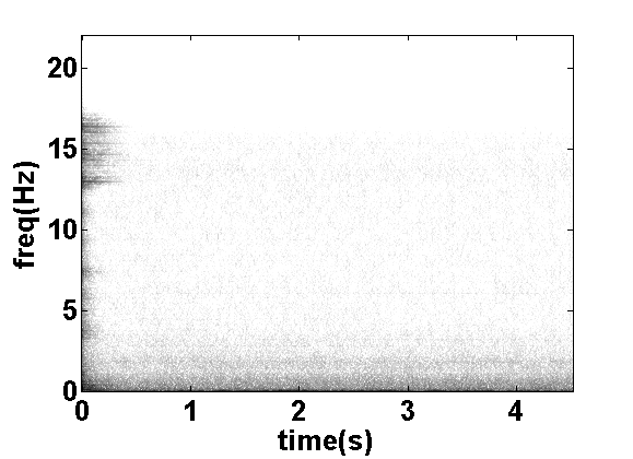
Figures 21 and 22 show a recorded guitar note on the guitar's high 'e' string and its Short-Time-Fourier-Transform (STFT), respectively. As shown, upon the onset of the note, all frequencies have energy. After the inital attack, most of the energy remains at the harmonic frequencies of the fundamental. The goal of excitation extraction is to remove the tonal components that ring after the initial onset and to reduce the energy during the onset at those components to match the general energy levels at other frequencies.
With the problem now graphically represented, we describe how the two different methods approach removal of harmonic peaks shown in the STFT. The inverse-filtering methods remove the harmonic peaks by inverse-filtering the signal with a comb-filter with peaks at the harmonic frequencies. The COLA methods remove the harmonic peaks by applying non-linear averaging to the magnitudes at each STFT frame of the signal.
The first method is the Matrix-Pencil Inverse-Filtering method [34]. It computes the sinusoidal components of a signal, using the Matrix-Pencil method, and performs inverse-filtering with the sinusoidal components to remove the tonal components leaving the excitation [35].
The second method, the Sines-Plus-Noise Inverse-Filtering method is similar to the Matrix-Pencil method, in that sinusoidal components of a model are computed, but instead of using the Matrix-Pencil method for computing the sinusoidal components, a generative sinusoidal model is used [36,37]. A residual signal is computed from subtracting from the original recording the sinusoidal signal. Inverse-filtering is then performed on the recording using a Digital Waveguide tuned for the recording where scaled versions of the residual and sinusoidal signals are added together to help remedy the notches created from inverse-filtering [38].
The third method, the Magnitude Spectrum Smoothing, uses STFT processing. Within each FFT window, a low-pass filter is applied to the magnitude spectrum of the window. The iFFT is then taken where the resulting time-signal is stored in a buffer for overlap-add [39].
The last method, the Statistical Spectral Interpolation method, similar to the MSS method, performs STFT processing and COLA reconstruction, but removes harmonic peaks by sampling new spectral magnitudes at the peaks according to a normal distribution with mean and covariance equal to those of magnitudes in the values surrounding the peak for each FFT frame [33].
As the literature shows, SSI produces the best psycho-acoustically sounding excitations. Here, we present the method in detail.
 |
 |
From a high-level viewpoint, the SSI method only modifies the magnitudes of the STFT of the guitar tone without affecting phase information. The method collects statistics on the magnitudes of frequencies surrounding harmonic peaks and uses these statistics to generate non-deterministic gain-changes for the magnitudes at these peaks, without modifying the phase. With inverse-filtering methods, modifying phase inevitably introduces artifacts. Thus, this method's primary goal is to minimally-alter the original tone.
The STFT is used for analyzing and modifying the original recorded
tone. The STFT can be seen as a sliding window that takes at each
sample-window a FFT of the windowed signal. The
transform of that windowed portion is then modified, and the
iFFT is then taken and saved in a buffer.
The window is then slid according to how much overlap is wanted. The
parameters for the STFT are the type of window used, the length of the
window and the number of samples the window slides by. Sample parameters
for the method are a Hamming window of length ![]() samples with
samples with
![]() overlap (hop size of
overlap (hop size of ![]() samples).
Though
samples).
Though ![]() samples with a
sampling-rate of
samples with a
sampling-rate of ![]() Hz is long (
Hz is long (
![]() ms),
pre-echo-distortion artifacts are remedied by starting the algorithm during the
onset of the recorded tone.
ms),
pre-echo-distortion artifacts are remedied by starting the algorithm during the
onset of the recorded tone.
Actual processing occurs at each window of the STFT. Consider each FFT window taken to be a frame for processing. Within each frame, the harmonic peaks of the recorded tone are attenuated. Harmonic peaks can be found using the Quadratically Interpolated FFT (QIFFT) method [40].
Assuming that the fundamental frequency of the recorded tone is at ![]() in Hz.
A bandwidth
in Hz.
A bandwidth ![]() in Hz is specified,
indicating the width of the peak.
Another bandwidth
in Hz is specified,
indicating the width of the peak.
Another bandwidth ![]() in Hz is specified indicating
the width of the interval used for statistics collecting with respect to
the fundamental frequency
in Hz is specified indicating
the width of the interval used for statistics collecting with respect to
the fundamental frequency ![]() . In using the SSI method for the recording
in Figure 21,
. In using the SSI method for the recording
in Figure 21,
![]() and
and
![]() . These
values ensure that the points used for statistics collecting do not reach into
the next harmonic peak but are large enough to obtain a reasonable mean
and standard deviation.
. These
values ensure that the points used for statistics collecting do not reach into
the next harmonic peak but are large enough to obtain a reasonable mean
and standard deviation.
For each harmonic ![]() with frequency
with frequency ![]() , the
following is defined and used for processing.
, the
following is defined and used for processing.
Define a set of indices, ![]() , whose frequency values satisfy
the following:
, whose frequency values satisfy
the following:
| (4) |
where ![]() corresponds to the frequency in Hz of the
corresponds to the frequency in Hz of the ![]() th FFT bin.
The values in
th FFT bin.
The values in ![]() correspond to indices within the current frame
whose frequencies lie within the specified band
correspond to indices within the current frame
whose frequencies lie within the specified band ![]() but outside the
band
but outside the
band ![]() centered around
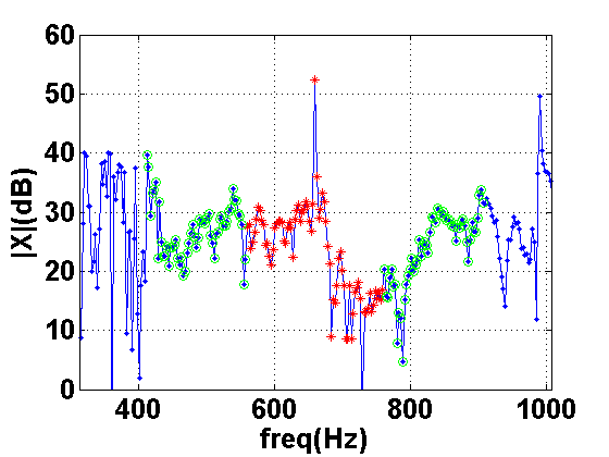
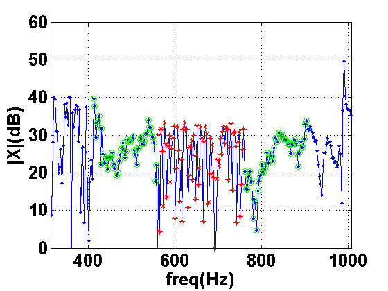
centered around ![]() . See the circled points
in Figures 27 and 28.
. See the circled points
in Figures 27 and 28.
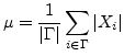
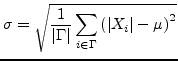
The mean and standard deviation of the
magnitude of values in FFT bins in ![]() are computed as follows:
are computed as follows:
Define the set of indices, ![]() , whose frequency values
satisfy the following:
, whose frequency values
satisfy the following:
| (7) |
Thus, for all bins with indices in ![]() , magnitude
values are modified to remove the observed peaks. This occurs as follows:
, magnitude
values are modified to remove the observed peaks. This occurs as follows:
For each
![]() , generate a value
, generate a value
![]() .
.
| (8) |
Figures 27 and 28 shows the points the algorithm uses
for statistics collecting and the points with gains altered. As shown,
the peak at ![]() Hz is entirely removed.
Hz is entirely removed.